Policy analysis and policy evaluation

Tutorial #1

Alexandre Grellet

Sciences Po Paris

Introducing myself

  • PhD student in economics, department of economics, Sciences Po;
  • Working on education policies;
  • Formerly at J-PAL Europe, a research institution specialized in the evaluation of public policies.

Your turn: who are you? Why did you choose this master?

Outline of the tutorials

1. Your questions first

Each class I will ask whether you have questions about the lectures.

  • If we have time \(\rightarrow\) answered live in class;
  • Otherwise \(\rightarrow\) by email.

2. Then the homework

  1. Random assignment to teams at the beginning of the class;
  2. 15 minutes of teamwork to agree on the answers (you are expected to have solved the problem set individually before the tutorial);
  3. Correction together \(\rightarrow\) each team gives the answers it agreed on.

Who are your class delegates ?

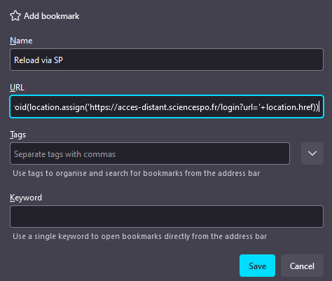
Tip to access papers faster

A useful browser bookmark

javascript:void(location.assign(
  'https://login.scpo.idm.oclc.org/login?url='
  + location.href))

How to use it

  1. Go to the article page (publisher, JSTOR, NBER…);
  2. Click your bookmark;
  3. Log in through the usual SP interface \(\rightarrow\) you get the paper.

Exercise #1

Exercise #1: the question

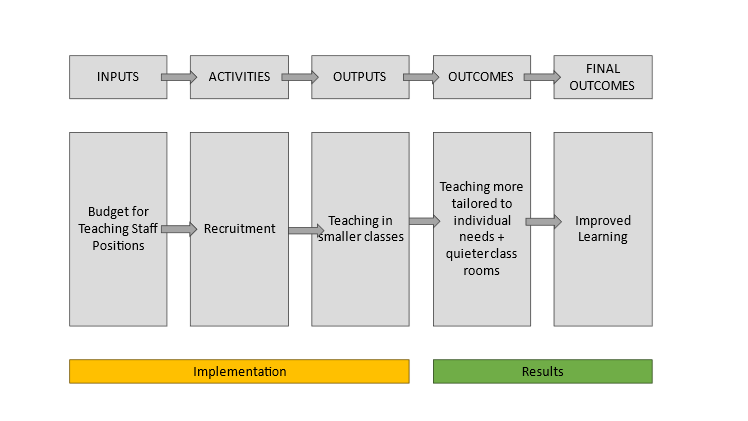
Theory of change: teacher positions

The French education ministry is considering whether to maintain the number of positions to recruit teachers in primary schools even though the number of students is falling.

  • Write the theory of change for this policy.
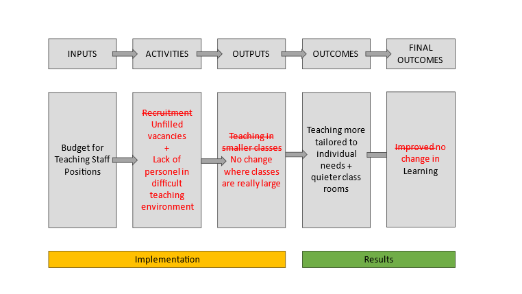
  • What could be possible implementation failures?
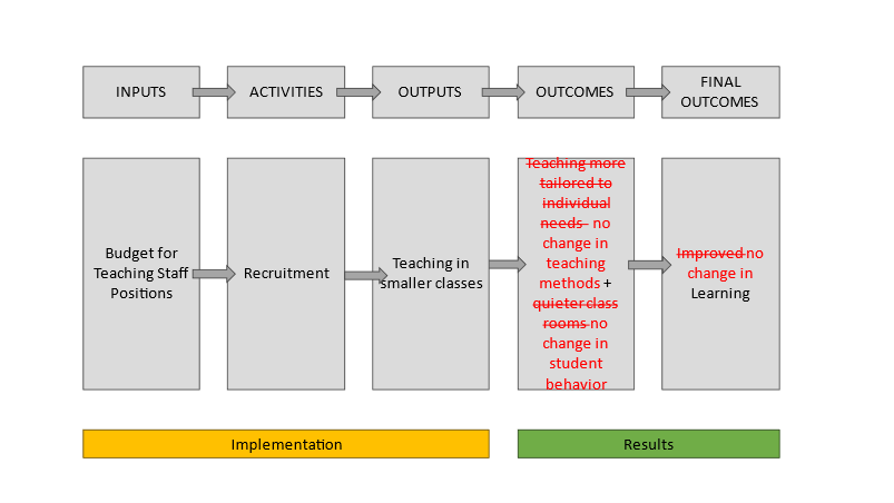
  • What could be possible theory failures?

Exercise #1: the theory of change

Exercise #1: possible implementation failures

Exercise #1: possible theory failures

Exercise #2

Exercise #2: the question

Franklin et al. (2024), UPSNP

Which parts of the paper by Franklin et al. (2024) on the UPSNP correspond to process evaluation and which to impact evaluation? Which data sources / statistical methods are used? What are their conclusions?

Exercise #2: answer

Process evaluation

\(\rightarrow\) the section “Program and Data”

  • tracks: how the program was implemented, the activities (registration, organization of the works), the outputs (take-up, employment);
  • Data: household survey data;
  • Purely descriptive;
  • Reveals good targeting, excellent take-up (97%).

Impact evaluation

\(\rightarrow\) the rest of the paper

  • Quantifies: impact on employment, amenities, commuting, labor markets;
  • Data: the same household survey;
  • Methods: statistics and regressions based on the RCT;
  • Results: amenities improve, total number of hours worked unchanged; private-sector crowd-out, wages \(\uparrow\).

Both answer different questions

Process evaluation asks was the program delivered as designed?, impact evaluation asks what difference did it make?

Exercise #3

Exercise #3: the question

De Neve et al. (2021), tax compliance

Do De Neve et al. (2021) mostly use qualitative or quantitative evidence? Describe what a mixed method approach could have looked like. How would it have improved the evaluation?

Exercise #3: answer

The evidence they use

  • Strictly quantitative: nationwide RCTs on administrative data;
  • Outcome observed: taxes paid (and filing);
  • Nothing on what people did with the letters, or what they thought of them.

What a qualitative arm would add

Focus groups / interviews of Belgian taxpayers, with varying demographics. This could have:

  • given a better sense of the cognitive costs behind the success of the simplified letter;
  • shown how people perceived the deterrence messages;
  • helped explain the counterintuitive results of the social-norms messaging.

Exercise #4

Exercise #4: the question

Banerjee et al. (2019), e-governance

Based on Banerjee et al. (2019), how would you do a cost-benefit analysis of the e-governance reform? If you had to compare it with Muralidharan et al. (2016) cited in Banerjee et al. (2019) p.4, what would be your conclusion regarding its cost-effectiveness?

Exercise #4: answer

Compute the costs

  • IT infrastructure (roll-out, maintenance);
  • Staff and training, heavier administrative burden;
  • Delayed payments to beneficiaries \(\rightarrow\) how do we value this?

Quantify the benefits

  • Reduced corruption / leakage;
  • Money saved for the state government budget;
  • Fewer ghost households on the rolls.

Cost-effective… for whom?

From the government’s perspective, the cost-benefit balance is positive and cost-effectiveness is very good. But what happens once we add the large costs borne by beneficiaries? Compare with the smartcards of Muralidharan et al. (2016), which increased payments to workers at no extra fiscal cost. Questions more generally the optimization problem for the state: maximize social welfare… but with which weights? And assuming what kind of preferences?

Exercise #5

Exercise #5: the question

Pons and Liegey (2019), door-to-door canvassing

A political party wants to increase electoral participation at regional elections in France, with a focus on socio-economically disadvantaged people, and in particular foreign-born citizens. To reach this goal, volunteers organize door-to-door visits to convey practical information about the elections, to urge people to vote and to encourage voting for their political party. Pons and Liegey (2018) evaluate the impact of this program.

Indicators to test

  1. How informed are people about local politics (region president, budget of the region, etc.)?
  2. Are immigrants more or less informed than citizens born in France?
  3. Where are migrants from, and how many from each place?
  4. How often were doors opened to canvassers?
  5. Do immigrants report receiving more canvassers than citizens born in France?

Exercise #5: loading the data

On Moodle, you have access to a subset of the data they gathered for their paper. Download it and load it in R.

### set your working directory below

# setwd(my path)

### Load libraries

library(arrow)
library(dplyr)
library(haven)

### Load the data

df <- read_parquet(
  "Pons_Liegey_dataset_short.parquet")

### Stata value labels:
### needed for `treatment == 0` to work
df <- zap_labels(df)

Exercise #5: summary table

We focus on baseline knowledge of local politics, so we keep only individuals in the control group who completed the survey, and build a summary table.

## Subset dataset to individuals who completed the survey
## And keep only individuals in the control group

sv <- df%>%
  filter(!is.na(surveycomplete) & treatment == 0)

## Summary statistics: basic summary

reg_pol <- sv%>%
  select(Q1_registered, Q7_knows_pres, Q8_knows_budget)

summary(reg_pol)
 Q1_registered    Q7_knows_pres    Q8_knows_budget 
 Min.   :0.0000   Min.   :-99.00   Min.   :0.0000  
 1st Qu.:1.0000   1st Qu.:-99.00   1st Qu.:0.0000  
 Median :1.0000   Median :  1.00   Median :0.0000  
 Mean   :0.8311   Mean   :-29.72   Mean   :0.4104  
 3rd Qu.:1.0000   3rd Qu.:  2.00   3rd Qu.:1.0000  
 Max.   :1.0000   Max.   :  3.00   Max.   :3.0000  
 NA's   :3        NA's   :18       NA's   :18      
## Summary statistics: improving layout

summary_table <- psych::describe(reg_pol) %>%   # keep only certain columns
  select(n, median, mean, min, max)

# need to add count for NAs manually
summary_table$NAs <- colSums(is.na(reg_pol))

kable(summary_table, digits = 2)
n median mean min max NAs
Q1_registered 456 1 0.83 0 1 3
Q7_knows_pres 441 1 -29.72 -99 3 18
Q8_knows_budget 441 0 0.41 0 3 18

Exercise #5: labelling for the barcharts

## Summary statistics: visualization

# look at the codes actually used
unique(reg_pol$Q1_registered)
[1]  1 NA  0
unique(reg_pol$Q7_knows_pres)
[1]   1   2 -99   3  NA -97
unique(reg_pol$Q8_knows_budget)
[1]  1  2  0  3 NA
# Give labels for barchart.
# case_when() reads top to bottom; anything unmatched (NA, -99, -97)
# falls through to the last line.
reg_pol <- reg_pol %>%
  mutate(
    know_registration = case_when(
      Q1_registered == 1 ~ "Registered",
      Q1_registered == 0 ~ "Not registered",
      TRUE               ~ "Doesn't know/answer"),

    know_pres = case_when(
      Q7_knows_pres == 1 ~ "Correct",
      Q7_knows_pres == 2 ~ "Partially correct",
      Q7_knows_pres == 3 ~ "Incorrect",
      TRUE               ~ "No answer"),

    # small trick to have categories in a meaningful order
    know_pres = factor(know_pres, levels = c("Correct",
                                             "Partially correct",
                                             "Incorrect",
                                             "No answer")),

    use_budget = if_else(is.na(Q8_knows_budget),
                         "No answer",
                         as.character(Q8_knows_budget)))

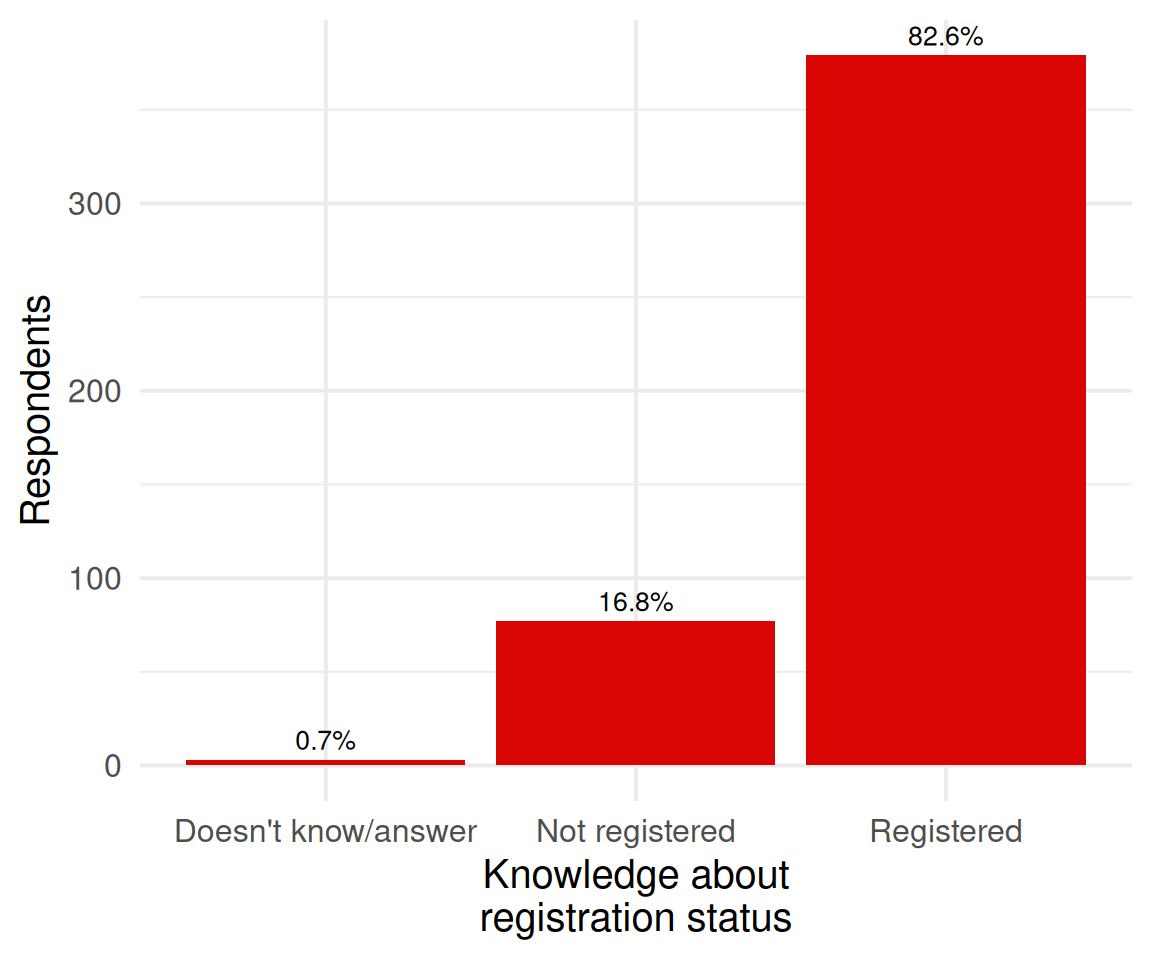
Exercise #5: knowledge about registration status

ggplot(reg_pol,
       aes(x = know_registration)) +
  geom_bar(fill = "#d90502") +
  geom_text(
    aes(label = scales::percent(after_stat(count)/sum(after_stat(count)), 
                                accuracy = 0.1)),
    stat = "count",
    vjust = -0.5,
    size = 3.5
  ) +
  labs(x = "Knowledge about\nregistration status",
       y = "Respondents")

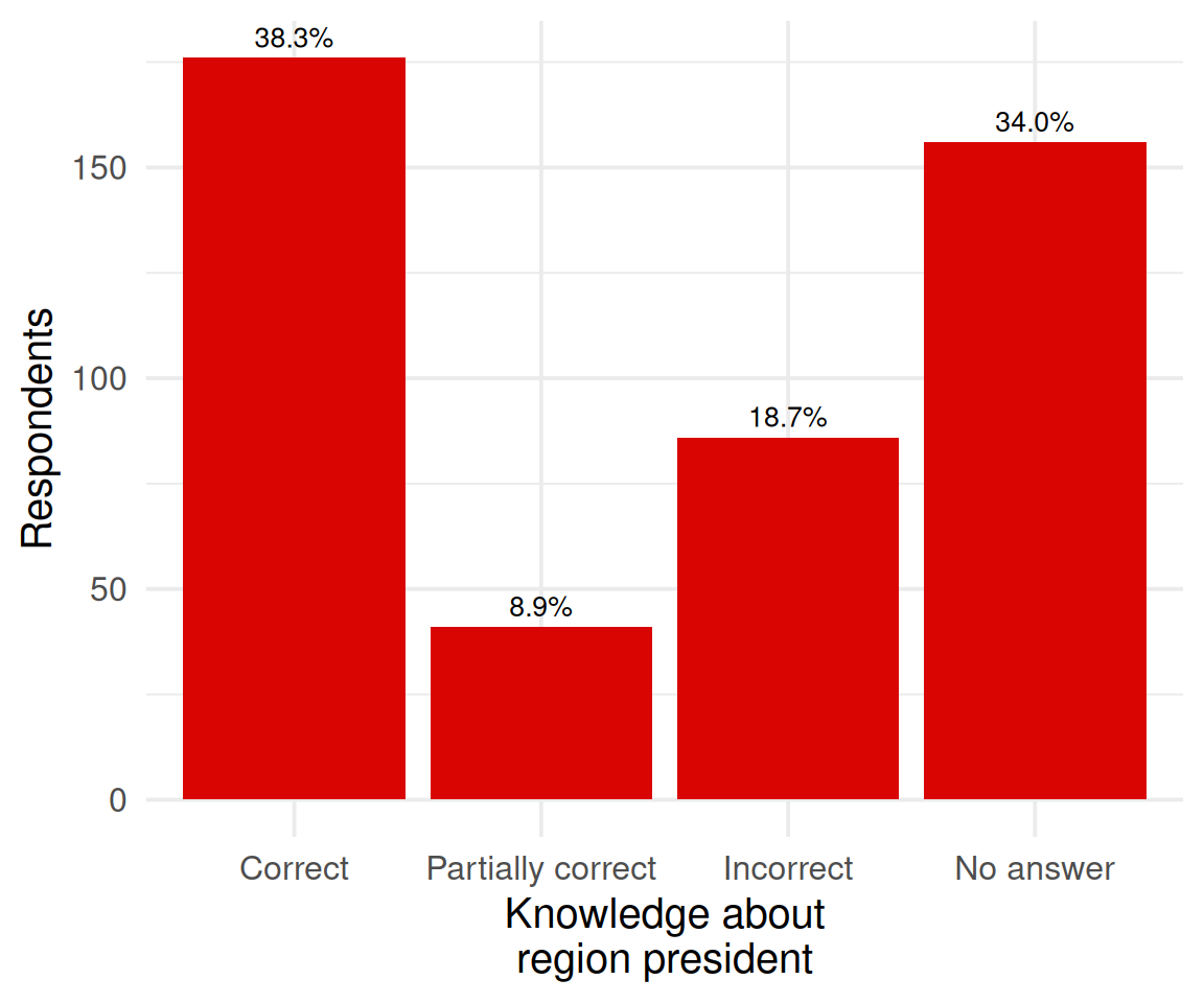
Exercise #5: knowledge about the region president

ggplot(reg_pol, aes(x = know_pres)) +
  geom_bar(fill = "#d90502") +
  geom_text(
    aes(label = scales::percent(after_stat(count)/sum(after_stat(count)), 
                                accuracy = 0.1)),
    stat = "count",
    vjust = -0.5,
    size = 3.5
  ) +
  labs(x = "Knowledge about\nregion president",
       y = "Respondents")

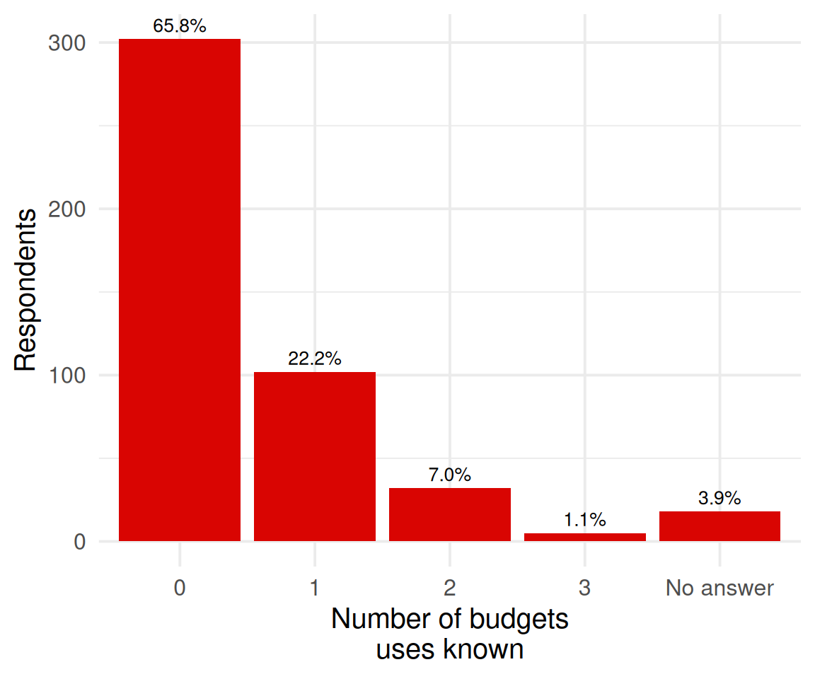
Exercise #5: knowledge about budget uses

ggplot(reg_pol,
       aes(x = use_budget)) +
  geom_bar(fill = "#d90502") +
  geom_text(
    aes(label = scales::percent(after_stat(count)/sum(after_stat(count)), 
                                accuracy = 0.1)),
    stat = "count",
    vjust = -0.5,
    size = 3.5
  ) + 
  labs(x = "Number of budgets\nuses known",
       y = "Respondents")

Exercise #5: simple averages

We can also look at simple averages.

## variables needed
# hint: using "==" can produce NAs, "%in%" never does

sv <- sv %>%
  mutate(
    registered_know = Q1_registered %in% 1,
    knows_pres      = Q7_knows_pres %in% 1,
    may_know_pres   = Q7_knows_pres %in% c(1, 2),
    #:> we consider here that people who don't want to answer actually
    # don't know whether they are registered, or are not registered
    budget          = if_else(is.na(Q8_knows_budget), 0, Q8_knows_budget))

## Share that know that they are registered
reg_know <- mean(sv$registered_know)

## Two ways of handling non-response on the president question.
# (a) drop non-respondents
pres <- sv %>%
  filter(!Q7_knows_pres %in% c(NA, -99, -97))

Pres_know_resp <- mean(pres$knows_pres)
part_know_resp <- mean(pres$may_know_pres)

# (b) extreme case: treat every non-respondent as not knowing.
#     This is the version quoted on the next slide.
Pres_know <- mean(sv$knows_pres)
part_know <- mean(sv$may_know_pres)

## Same choice for the budget question
bud_know_resp <- mean(sv$Q8_knows_budget, na.rm = TRUE)  # (a) respondents only
bud_know      <- mean(sv$budget)                         # (b) non-response = 0

Exercise #5: how informed are people?

Before treatment, respondents are poorly informed about regional politics.

82.6%

know that they are registered to vote

38.3%

name the region president correctly, just after the elections

47.3%

are correct or approximately correct about the president

0.39

uses of the regional budget known, on average

Non-response matters

These figures count every non-respondent as not knowing. Keeping only respondents instead gives 58.1% for the president and 0.41 budget uses.

Exercise #5: immigrants vs France-born

Same code as above, but always differentiating by origin.

## One group_by() replaces building the two halves of the table by hand

out.tab <- sv %>%
  filter(immigrant %in% c(0, 1)) %>%
  group_by(Immigrant = if_else(immigrant == 1, "Yes", "No")) %>%
  summarise(
    Registered              = mean(registered_know),
    President               = mean(knows_pres),
    `Approximate President` = mean(may_know_pres),
    Budget                  = mean(budget),
    .groups                 = "drop")

# Print the summary statistics table
kable(out.tab,
      caption = "Summary Statistics by origin",
      align   = "c",
      digits  = 3)
Summary Statistics by origin
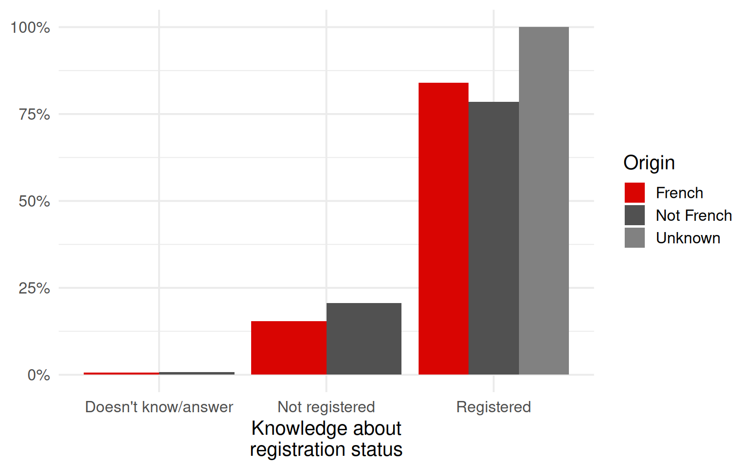
Immigrant Registered President Approximate President Budget
No 0.840 0.409 0.496 0.418
Yes 0.785 0.314 0.413 0.331

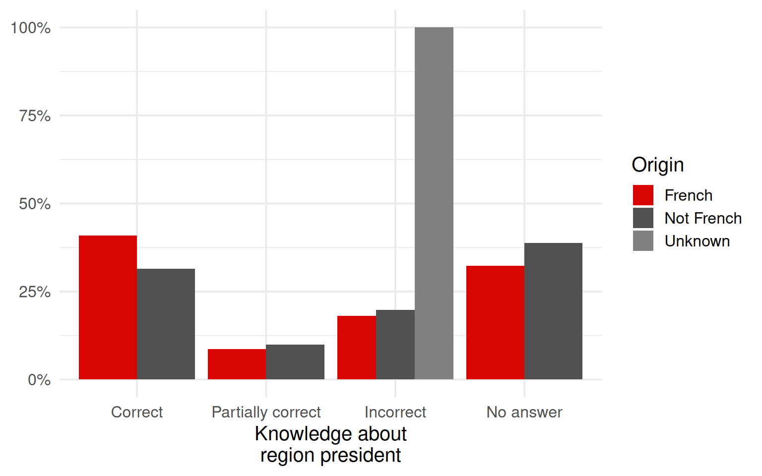
Exercise #5: barcharts by origin

We could also look at the barcharts:

# Exactly the same labelling as before, now also recoding the origin.
# Note `know_pres_lab`: `knows_pres` above is the TRUE/FALSE version and
# we do not want to overwrite it.

sv <- sv %>%
  mutate(
    know_registration = case_when(
      Q1_registered == 1 ~ "Registered",
      Q1_registered == 0 ~ "Not registered",
      TRUE               ~ "Doesn't know/answer"),

    know_pres_lab = case_when(
      Q7_knows_pres == 1 ~ "Correct",
      Q7_knows_pres == 2 ~ "Partially correct",
      Q7_knows_pres == 3 ~ "Incorrect",
      TRUE               ~ "No answer"),

    know_pres_lab = factor(know_pres_lab, levels = c("Correct",
                                                     "Partially correct",
                                                     "Incorrect",
                                                     "No answer")),

    use_budget = if_else(is.na(Q8_knows_budget),
                         "No answer",
                         as.character(Q8_knows_budget)),

    origin = case_when(
      immigrant == 0 ~ "French",
      immigrant == 1 ~ "Not French",
      TRUE           ~ "Unknown"))

Exercise #5: registration status, by origin

## Compute percentages of observations
## in each category, by origin.
sv_plot <- sv %>%
  count(origin, know_registration,
        name = "count") %>%
  group_by(origin) %>%
  mutate(percentage = count / sum(count)) %>%
  ungroup()

ggplot(sv_plot,
       aes(x = know_registration,
           y = percentage,
           fill = origin)) +
  geom_col(position = position_dodge()) +
  scale_y_continuous(labels = scales::percent) +
  labs(x = "Knowledge about\nregistration status",
       y = NULL) +
  scpo_fill

Exercise #5: region president, by origin

sv_plot <- sv %>%
  count(origin, know_pres_lab,
        name = "count") %>%
  group_by(origin) %>%
  mutate(percentage = count / sum(count)) %>%
  ungroup()

ggplot(sv_plot,
       aes(x = know_pres_lab,
           y = percentage,
           fill = origin)) +
  geom_col(position = position_dodge()) +
  scale_y_continuous(labels = scales::percent) +
  labs(x = "Knowledge about\nregion president",
       y = NULL) +
  scpo_fill

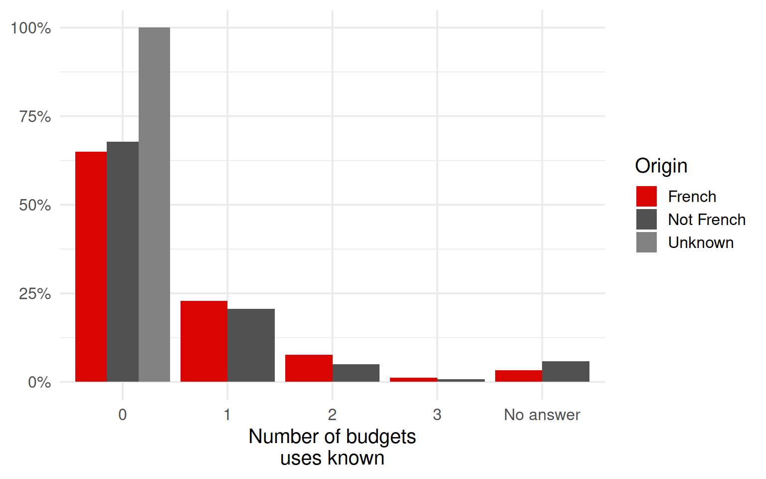
Exercise #5: budget uses, by origin

sv_plot <- sv %>%
  count(origin, use_budget,
        name = "count") %>%
  group_by(origin) %>%
  mutate(percentage = count / sum(count)) %>%
  ungroup()

ggplot(sv_plot,
       aes(x = use_budget,
           y = percentage,
           fill = origin)) +
  geom_col(position = position_dodge()) +
  scale_y_continuous(labels = scales::percent) +
  labs(x = "Number of budgets\nuses known",
       y = NULL) +
  scpo_fill

Exercise #5: where are migrants from?

Migrants come from regions all over the world: Maghreb, , Asia, Africa, South America, Western Europe, Eastern Europe, Middle East, North America. We can count people from different regions:

regions <- df %>%
  filter(immigrant == 1) %>%
  mutate(birth_region = if_else(birth_region == "", "Unknown", birth_region))

# count() does in one line what a for() loop over regions would do,
# and returns a table we can sort and print.
regions <- regions %>%
  count(birth_region, name = "Number") %>%
  mutate(`Share total (%)` = 100 * Number / nrow(regions)) %>%
  arrange(desc(Number))

kable(regions, align = "lrr", digits = 2)
birth_region Number Share total (%)
Maghreb 2042 38.15
Africa 1546 28.89
Asia 1050 19.62
Western Europe 222 4.15
South America 217 4.05
Eastern Europe 155 2.90
Middle East 112 2.09
North America 7 0.13
Unknown 1 0.02

Exercise #5: how often were doors opened?

Watch the unit of observation

The number of doors canvassed and opened is only known at the building level. We must therefore keep one row per visited building.

## Keep only one row per building and relevant variables

buildings <- df %>%
  group_by(cluster) %>%
  slice(1) %>%
  ungroup() %>%
  select(cluster,
         actualtreatment,
         knocked_doors,
         opened_doors)

## Look at the number of doors canvassed and the share that was opened
##:> computed on `buildings`, not on `df`: one row per building, so
##     each building is counted once rather than once per resident.

building_visited <- sum(buildings$actualtreatment, na.rm = TRUE)
knocked_doors    <- sum(buildings$knocked_doors,   na.rm = TRUE)
share_open       <- sum(buildings$opened_doors, na.rm = TRUE) /
                    sum(buildings$knocked_doors, na.rm = TRUE)

Exercise #5: how often were doors opened?

608

buildings visited by canvassers

9,070

doors knocked at

48.9%

of those doors were opened

Exercise #5: do immigrants report more canvassers?

Two restrictions, and one problem

We keep only households randomized to receive a canvasser (to avoid capturing canvassers outside the study) and individuals who completed the survey (only they can report a visit). This second restriction induces selection: how would you deal with it?

# Restrict dataset to buildings both visited by canvassers and
# part of the survey + keep only individuals who completed survey
# This last part induces selection. How would you deal with it ?

build <- df %>%
  filter(actualtreatment == 1 & surveycomplete == 1)

# Look at the label for visit reports in the survey
unique(build$Q9a_visit_activists)

# Code variable for being visited
build <- build %>%
  mutate(visited = Q9a_visit_activists %in% c(1, 2))

# Look at whether canvassers were received
share_visited <- mean(build$visited) * 100

# filter() drops the rows where `immigrant` is missing; subsetting with
# build[build$immigrant == 0, ] would instead keep them as all-NA rows
# and inflate the denominator.
shares <- build %>%
  filter(immigrant %in% c(0, 1)) %>%
  group_by(immigrant) %>%
  summarise(share = mean(visited) * 100, n = n(), .groups = "drop")

share_visited_F  <- shares$share[shares$immigrant == 0]
share_visited_NF <- shares$share[shares$immigrant == 1]

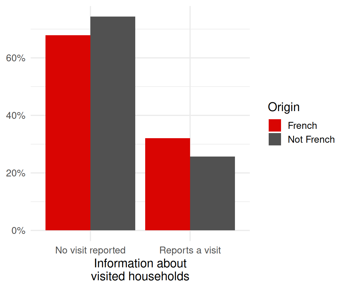
Exercise #5: visualization

## Visualization

build <- build %>%
  filter(immigrant %in% c(0, 1)) %>%
  mutate(
    # recode origin of individuals
    origin = case_when(
      immigrant == 0 ~ "French",
      immigrant == 1 ~ "Not French",
      TRUE           ~ "Unknown"),
    # give meaningful label to "visited"
    visited_labeled = if_else(
      visited,
      "Reports a visit",
      "No visit reported"))

# compute share visited per origin
build_plot <- build %>%
  count(origin, visited_labeled,
        name = "count") %>%
  group_by(origin) %>%
  mutate(percentage = count / sum(count)) %>%
  ungroup()

ggplot(build_plot,
       aes(x = visited_labeled,
           y = percentage,
           fill = origin)) +
  geom_col(position = position_dodge()) +
  scale_y_continuous(labels = scales::percent) +
  labs(x = "Information about\nvisited households",
       y = NULL) +
  scpo_fill

Exercise #5: do immigrants report more canvassers?

Most households did not report any canvasser.

30.4%

of all households report a visit

32.1%

of France-born citizens report a visit

25.7%

of immigrants report a visit

Meaningful, but not significant

The gap differs meaningfully along origin: is that surprising to you, or could it be expected? Note that the difference is not statistically significant.

Exercise #5: regression

summary(lm(visited ~ immigrant, data = build))

Call:
lm(formula = visited ~ immigrant, data = build)

Residuals:
    Min      1Q  Median      3Q     Max 
-0.3211 -0.3211 -0.2569  0.6789  0.7431 

Coefficients:
            Estimate Std. Error t value Pr(>|t|)    
(Intercept)  0.32107    0.02661  12.064   <2e-16 ***
immigrant   -0.06419    0.05149  -1.247    0.213    
---
Signif. codes:  0 '***' 0.001 '**' 0.01 '*' 0.05 '.' 0.1 ' ' 1

Residual standard error: 0.4602 on 406 degrees of freedom
Multiple R-squared:  0.003813,  Adjusted R-squared:  0.00136 
F-statistic: 1.554 on 1 and 406 DF,  p-value: 0.2133

References

De Neve, Jan-Emmanuel, Clément Imbert, Johannes Spinnewijn, Teodora Tsankova, and Maarten Luts. 2021. “How to Improve Tax Compliance? Evidence from Population-Wide Experiments in Belgium.” Journal of Political Economy 129 (5): 1425–63. https://doi.org/10.1086/713096.
Franklin, Simon, Clément Imbert, Girum Abebe, and Carolina Mejia-Mantilla. 2024. “Urban Public Works in Spatial Equilibrium: Experimental Evidence from Ethiopia.” American Economic Review 114 (5): 1382–414. https://doi.org/10.1257/aer.20220471.
Pons, Vincent, and Guillaume Liegey. 2019. “Increasing the Electoral Participation of Immigrants: Experimental Evidence from France.” The Economic Journal 129 (617): 481–508. https://doi.org/10.1111/ecoj.12584.

Appendix

First-Order Stochastic Dominance (FOSD)

Definition

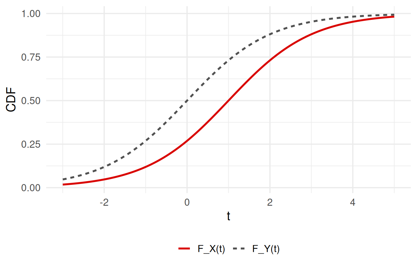
A random variable \(X\) first-order stochastically dominates \(Y\) if

\[F_X(t) \le F_Y(t)\quad \forall\, t\in\mathbb{R},\]

with strict inequality for some \(t\).

  • Intuition: \(X\) yields weakly higher outcomes than \(Y\) at every threshold \(t\);
  • Preference: any decision-maker with increasing utility prefers \(X\) to \(Y\).

Graphical intuition (CDF ordering)

\(F_X\) (dashed) lies everywhere at or below \(F_Y\) (solid) \(\Rightarrow\) \(X\) FOSD \(Y\).

// allow image sizing using percentage remark.macros.scale = function (percentage) { var url = this; return ''; };