Policy analysis and policy evaluation

Tutorial #3

Alexandre Grellet

Department of Economics, SciencesPo

Exercise #1: Card and Krueger (1994): minimum wage

Exercise #1

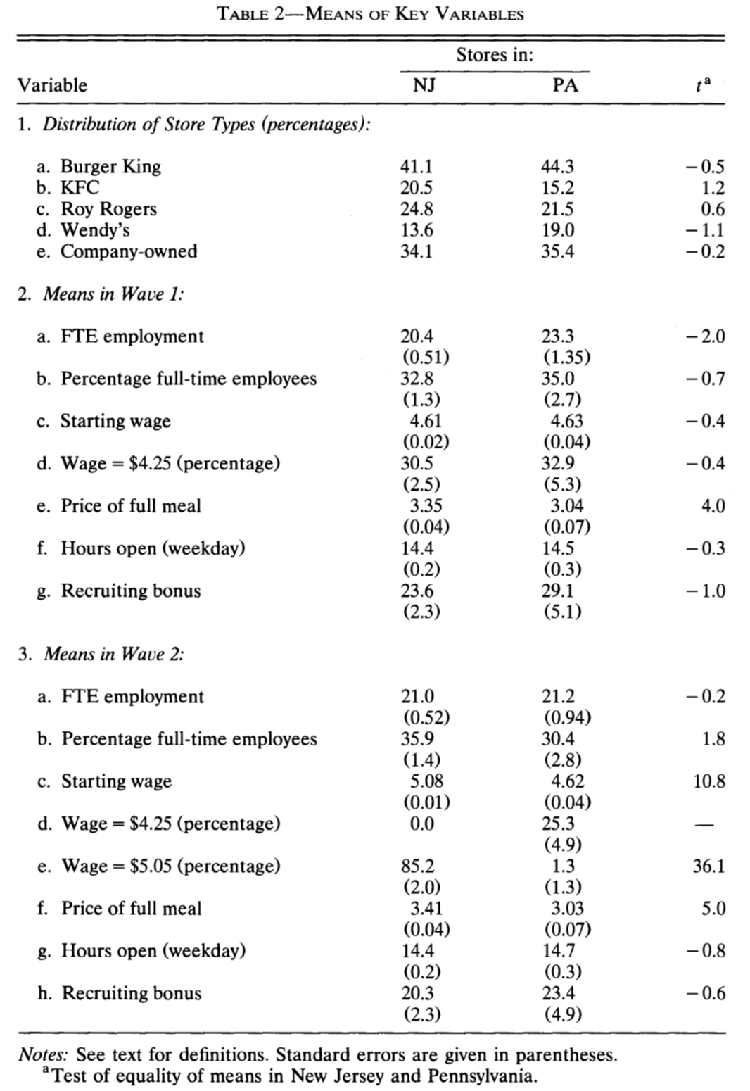
Card and Krueger (1994) study the effect of minimum wage laws on employment. They carried out two waves of a phone survey of fast-food stores in New Jersey and Pennsylvania, before (wave 1) and after (wave 2) the introduction of a $5.05 minimum wage in New Jersey. Table 2 summarizes the key outcomes used in the study across the two states.

Question

What are the statistics presented in each column?
Exercise #1: the columns

  • Columns NJ and PA: means of each variable in the two states, with their standard errors in parentheses (for Panels 2 and 3).
  • Column \(t\): t-statistic of the test of equality of means between New Jersey and Pennsylvania.

Exercise #1: t-statistic

Question

How is the t-statistic for the starting wage in Wave 1 (Panel 2) computed?

Exercise #1: t-statistic

The two samples (NJ and PA stores) are independent, so we use the formula from Tutorial 2:

\[t = \frac{\overline{Y}_{NJ} - \overline{Y}_{PA}}{\sqrt{SE(\overline{Y}_{NJ})^2 + SE(\overline{Y}_{PA})^2}}\]

In R:

t_wage_w1 <- (4.61 - 4.63) / sqrt(0.02^2 + 0.04^2)
t_wage_w1
[1] -0.4472136

We find the \(-0.4\) reported in the table.

Exercise #1: conclusions

Question

Using the 5% significance level, which conclusions would you draw from this table regarding the effect of minimum wage laws on starting wages? Employment?

Exercise #1: conclusions

tstat <- function(m1, se1, m2, se2) (m1 - m2) / sqrt(se1^2 + se2^2)

round(c(wage_w1 = tstat(4.61, 0.02, 4.63, 0.04),
        wage_w2 = tstat(5.08, 0.01, 4.62, 0.04),
        fte_w1  = tstat(20.4, 0.51, 23.3, 1.35),
        fte_w2  = tstat(21.0, 0.52, 21.2, 0.94)), 2)
wage_w1 wage_w2  fte_w1  fte_w2 
  -0.45   11.16   -2.01   -0.19 

(We get likely 11.2 instead of 10.8 for wages in wave 2 because the table rounds the standard errors.)

  • Starting wages: identical in both states before the law (\(|t| = 0.4 < 1.96\)), much higher in NJ after the law (\(t \gg 1.96\)): a clear, significant effect at the 5% level.
  • Employment: looks a bit weird. Employment is lower in NJ before the law (\(|t| = 2.0 > 1.96\), borderline) and the same after. The authors conclude that they find no negative effect of the minimum wage on employment, but the pre-law difference casts doubt on the comparability of the two states.

Exercise #1: store types

Question

In Panel 1 the authors compare the market share of different store types at baseline across the two states. What are the lessons from this exercise?

Exercise #1: store types

  • The authors want to check that the differences in wages or employment between states are not due to differences in store types: e.g. if Burger King had a large share in NJ and a more generous wage policy.
  • None of the differences in Panel 1 is significant (all \(|t| < 1.96\)), which suggests that the two states are comparable in terms of observable characteristics. This is the same logic as the balance table of Tutorial 2.

Teaser

There is a more interesting assumption that Card and Krueger are using: you will study it next semester. Any idea?

They assume that, without the law, employment in NJ would have evolved like employment in PA (parallel trends).

Exercise #1: regression

Question

Using only information present in this table, how would you test the effect of minimum wages on employment with a regression?

Exercise #1: regression

Post-law comparison (wave 2 only):

\[Y_i = \beta_0 + \beta_1 NJ_i + \varepsilon_i\]

where \(Y_i\) is wages or employment in wave 2 in restaurant \(i\) and \(NJ_i\) a dummy equal to one if restaurant \(i\) is in New Jersey. \(\hat\beta_1\) is the difference in means between NJ and PA.

Controlling for store characteristics (e.g. company-owned):

\[Y_i = \beta_0 + \beta_1 NJ_i + \beta_2 Company_i + \varepsilon_i\]

Difference in differences, using wave 1 as well:

\[Y_{it} = \beta_0 + \beta_1 NJ_i \times Wave2_t + \beta_2 NJ_i + \beta_3 Wave2_t + \varepsilon_{it}\]

where \(Wave2_t\) is a dummy equal to one for wave 2. \(\hat\beta_1\) is the change in NJ minus the change in PA:

did_fte <- (21.0 - 20.4) - (21.2 - 23.3)
did_fte
[1] 2.7

FTE employment increased by about 2.7 employees per store in NJ relative to PA.

Exercise #2: Andrabi et al. (2011): value-added models

Exercise #2

Andrabi et al. (2011) discuss the value-added model which is often used to estimate the effect of school or teacher characteristics, using the example of private schools in Pakistan. They first regress \(y_{it}\), English test scores in third grade for individual \(i\), on a dummy \(P_{it}\) equal to one if individual \(i\) is in private school in third grade:

\[y_{it} = \alpha_0 + \alpha_1 P_{it} + u_{it}\]

Question

What is the issue with this regression? What would you do about it?

Exercise #2: omitted variable bias

  • Selection into private schools: being in a private school is probably positively correlated with parental income, which correlates with parental education, which correlates with parental investments in their children (books, help with homework…), which increase test scores.
  • \(P_{it}\) is correlated with \(u_{it}\): \(\hat\alpha_1\) captures the effect of private schools and of everything that comes with being in a private school. It is biased upwards.

What to do: control for the omitted variables we observe (parental education, wealth, …), or better, find a source of variation in \(P_{it}\) unrelated to \(u_{it}\) (a lottery for school places, for instance).

Exercise #2: controls

They follow up with a regression:

\[y_{it} = \alpha_0 + \alpha_1 P_{it} + \alpha_2 X_{it} + u_{it}\]

Questions
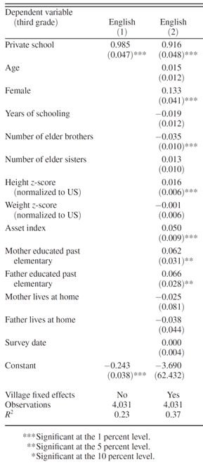
  • What do the stars mean next to the standard errors?
  • What does this table suggest regarding the impact of private schools on test scores?

Exercise #2: stars

The stars indicate the significance level at which we reject \(H_0\): coefficient \(= 0\) (see the notes below the table):

  • ***: p-value \(< 0.01\), i.e. \(|t| > 2.58\)
  • **: p-value \(< 0.05\), i.e. \(|t| > 1.96\)
  • *: p-value \(< 0.10\), i.e. \(|t| > 1.64\)
t_vals <- c(private = 0.916 / 0.048,
            mother_educ = 0.062 / 0.031,
            age = 0.015 / 0.012)
round(t_vals, 2)
    private mother_educ         age 
      19.08        2.00        1.25 
round(2 * (1 - pnorm(abs(t_vals))), 3) # p-values
    private mother_educ         age 
      0.000       0.046       0.211 

Exercise #2: what the table suggests

  • Many controls are included, among them parental education and wealth, which matter for test scores (significant coefficients, \(R^2\) goes from 0.23 to 0.37).
  • But the coefficient on private school barely moves (0.985 \(\rightarrow\) 0.916): maybe there is not that much selection into private schools?
  • Careful: this only rules out selection on the variables we observe. Child ability or motivation are still in \(u_{it}\).

Exercise #2: lagged value added

They now estimate what they call a lagged value-added model by including test scores at the beginning of school (\(y_{it-1}\)) in the equation:

\[y_{it} = \alpha_0 + \alpha_1 P_{it} + \beta y_{it-1} + u_{it}\]

Questions

Why can \(y_{it-1}\) be a good control to add? Why is it called value added?

Exercise #2: lagged value added

  • Previous test scores are a good proxy for child ability, but also for all other inputs received before (from parents, previous schools…).
  • They also matter to get into private schools: another good control for selection.
  • Value added: conditional on the initial level \(y_{it-1}\), \(\alpha_1\) measures how much the private school adds to the child’s learning during the year, rather than the level of the students it attracts.

Going further: the restricted model

Exercise #3: Coding exercise: Imbert (2013)

Exercise #3

Imbert (2013) decomposes earnings inequality between the public and private sectors in Vietnam. You will find the dataset from his paper on Moodle. You will use this data, focusing on log hourly deflated earnings (lhearnings1def), to estimate the returns to education through a regression similar to the Mincer model (Mincer 1974).

In the following questions, you should focus on estimating the causal impact of education on earnings.

Loading the data

### Set your working directory below
# setwd(my_path)

### Load libraries
library(arrow)
library(dplyr)
library(haven)
library(ggplot2)

### Load the data
df <- read_parquet("Imbert_2013_data.parquet")

# remove stata labels and haven_labelled type
df <- zap_labels(df)

A first look at the data

nrow(df)
[1] 39071
sum(!is.na(df$lhearnings1def))
[1] 7091
  • The survey covers all members of the households, but earnings are only observed for 7091 wage earners. lm() silently drops the other observations.
  • To make sure all our regressions use the same sample, we keep wage earners only:
df_w <- df %>% filter(!is.na(lhearnings1def))

Exercise #3: years of education

Question

First, estimate the relationship between log earnings and levels of education using a regression (command lm). How should you interpret the coefficients for these levels of education?

Exercise #3: years of education

grade measures the number of years of education:

reg_grade <- lm(lhearnings1def ~ grade, data = df_w)
summary(reg_grade)

Call:
lm(formula = lhearnings1def ~ grade, data = df_w)

Residuals:
    Min      1Q  Median      3Q     Max 
-3.4587 -0.3511 -0.0007  0.3519  3.3276 

Coefficients:
            Estimate Std. Error t value Pr(>|t|)    
(Intercept) 1.069973   0.018387   58.19   <2e-16 ***
grade       0.064504   0.001982   32.55   <2e-16 ***
---
Signif. codes:  0 '***' 0.001 '**' 0.01 '*' 0.05 '.' 0.1 ' ' 1

Residual standard error: 0.583 on 7089 degrees of freedom
Multiple R-squared:   0.13, Adjusted R-squared:  0.1299 
F-statistic:  1060 on 1 and 7089 DF,  p-value: < 2.2e-16

Exercise #3: interpretation

The regression is log-linear: the coefficient is a change in log earnings, which we can interpret as a percentage change.

  • One more year of education is associated with 0.065 more log points of hourly earnings, i.e. approximately 6.5% higher hourly earnings.
  • The approximation \(\log(1 + x) \approx x\) is good for small \(x\) (an implication of first-order Taylor approximations). The exact percentage change is

\[ \frac{e^{1+(\text{grade} + x)\cdot \widehat \beta}}{e^{1+\text{grade}\cdot \widehat \beta}} -1 = e^{x\hat\beta} - 1\]

For a one-year increase in education, that is:

exp(coef(reg_grade)["grade"]) - 1
     grade 
0.06662983 
  • The constant is the predicted log earnings of a worker with zero years of education.
  • This is a correlation: nothing guarantees that it is the causal effect of education (see next question).

Exercise #3: levels of education

We can also use the highest diploma (degree) and let each level have its own coefficient. The 708 workers with a missing diploma all have fewer than 5 years of education: they have no diploma.

df_w <- df_w %>%
  mutate(diploma = factor(coalesce(degree, 0), levels = 0:4,
                          labels = c("No diploma", "Primary", "Lower secondary",
                                     "Upper secondary", "Post-secondary")))

reg_diploma <- lm(lhearnings1def ~ diploma, data = df_w)
round(coef(summary(reg_diploma)), 3)
                       Estimate Std. Error t value Pr(>|t|)
(Intercept)               1.305      0.017  76.212        0
diplomaPrimary            0.125      0.022   5.682        0
diplomaLower secondary    0.239      0.021  11.125        0
diplomaUpper secondary    0.441      0.022  20.215        0
diplomaPost-secondary     0.966      0.025  38.425        0

Exercise #3: levels of education

  • Each coefficient is the difference in mean log earnings between workers with this diploma and the reference category (no diploma).
  • For large coefficients the approximation is bad: workers with a post-secondary degree do not earn 97% more, but:
round(exp(coef(reg_diploma)[-1]) - 1, 3)
        diplomaPrimary diplomaLower secondary diplomaUpper secondary 
                 0.133                  0.270                  0.554 
 diplomaPost-secondary 
                 1.628 
  • Why use diplomas? Returns may not be linear in years (diplomas have a value of their own), and grade stops at 12: the 910 workers with a post-secondary degree all have grade = 12.

Exercise #3: omitted variable bias

Question

Are you worried about omitted variable bias when using this model?

Exercise #3: omitted variable bias

Yes! Any variable that affects earnings and is correlated with education biases our estimate:

  • Ability, motivation, family background: positively correlated with education and with earnings \(\Rightarrow\) the coefficient is biased upwards.
  • Experience: at a given age, people who studied longer have spent fewer years on the labor market. Experience is negatively correlated with education and positively with earnings \(\Rightarrow\) the coefficient is biased downwards.
cor(df_w$grade, df_w$exp)
[1] -0.2553208

The omitted variable bias formula

Exercise #3: the Mincer equation

The Mincer equation (Mincer 1974) predicts that wages should be a function of both education and experience:

\[Y_i = \beta_0 + \beta_1 \times Education_i + \beta_2 \times Experience_i + \varepsilon_i\]

Question

Regress log hourly wages on education and experience (exp) of individuals. Discuss this regression.

Exercise #3: the Mincer equation

reg_exp <- lm(lhearnings1def ~ grade + exp, data = df_w)
summary(reg_exp)

Call:
lm(formula = lhearnings1def ~ grade + exp, data = df_w)

Residuals:
    Min      1Q  Median      3Q     Max 
-3.6901 -0.3343  0.0111  0.3486  3.3179 

Coefficients:
             Estimate Std. Error t value Pr(>|t|)    
(Intercept) 0.8714748  0.0234994   37.09   <2e-16 ***
grade       0.0713851  0.0020246   35.26   <2e-16 ***
exp         0.0073899  0.0005551   13.31   <2e-16 ***
---
Signif. codes:  0 '***' 0.001 '**' 0.01 '*' 0.05 '.' 0.1 ' ' 1

Residual standard error: 0.5759 on 7088 degrees of freedom
Multiple R-squared:  0.1512,    Adjusted R-squared:  0.151 
F-statistic: 631.5 on 2 and 7088 DF,  p-value: < 2.2e-16

Exercise #3: discussion

  • The coefficient on education increases from 0.0645 to 0.0714: as expected, omitting experience biased it downwards.
  • One more year of experience is associated with 0.7% higher hourly earnings, holding education constant.
  • exp is potential experience: for 93% of workers, it is exactly age - years of education - 6. It does not account for unemployment spells or time out of the labor force.
mean(df_w$exp == df_w$age - df_w$grade - 6)
[1] 0.9311804
  • Ability is still omitted: we cannot interpret \(\hat\beta_1\) as causal yet.

Exercise #3: experience and earnings

Questions

Plot the relationship between experience and log earnings. Pay attention to include the regression line. What can you say? Do you think we should add a term for \(\text{experience}^2\) in the regression?

Hint: you can try to use the loess method in geom_smooth to better observe the relationship between earnings and experience.

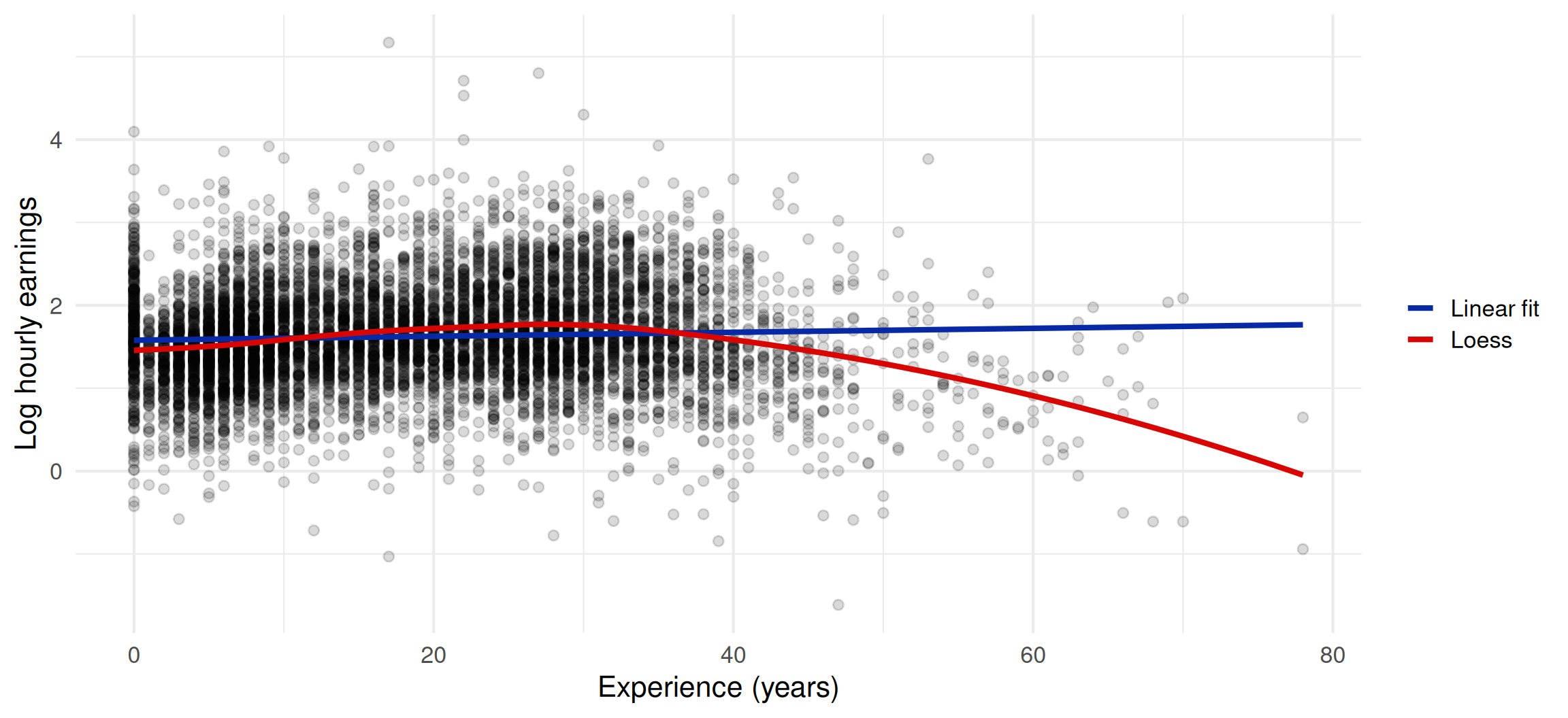
Exercise #3: experience and earnings

ggplot(df_w, aes(x = exp, y = lhearnings1def)) +
  geom_point(alpha = 0.15) +
  geom_smooth(aes(colour = "Linear fit"), method = "lm", formula = y ~ x, se = FALSE) +
  geom_smooth(aes(colour = "Loess"), method = "loess", formula = y ~ x, se = FALSE) +
  scale_colour_manual(name = NULL, values = c("Linear fit" = "#0729a6", "Loess" = "#d90502")) +
  labs(x = "Experience (years)", y = "Log hourly earnings") +
  theme_minimal(base_size = 16)

Exercise #3: experience and earnings

  • The linear fit is almost flat: it suggests that experience barely matters.
  • The loess curve shows a concave relationship: earnings increase with experience during the first part of the career, then flatten and decrease for the most experienced workers.
  • A straight line cannot capture this: we should add \(\text{experience}^2\) (this is the standard Mincer equation).

\[Y_i = \beta_0 + \beta_1 Educ_i + \beta_2 Exp_i + \beta_3 Exp_i^2 + \varepsilon_i\]

We expect \(\beta_2 > 0\) and \(\beta_3 < 0\).

Exercise #3: adding experience squared

reg_exp2 <- lm(lhearnings1def ~ grade + exp + I(exp^2), data = df_w)
summary(reg_exp2)

Call:
lm(formula = lhearnings1def ~ grade + exp + I(exp^2), data = df_w)

Residuals:
    Min      1Q  Median      3Q     Max 
-3.4282 -0.3360  0.0075  0.3352  3.2371 

Coefficients:
              Estimate Std. Error t value Pr(>|t|)    
(Intercept)  6.946e-01  2.493e-02   27.86   <2e-16 ***
grade        6.987e-02  1.981e-03   35.28   <2e-16 ***
exp          3.362e-02  1.538e-03   21.86   <2e-16 ***
I(exp^2)    -5.884e-04  3.228e-05  -18.23   <2e-16 ***
---
Signif. codes:  0 '***' 0.001 '**' 0.01 '*' 0.05 '.' 0.1 ' ' 1

Residual standard error: 0.5629 on 7087 degrees of freedom
Multiple R-squared:  0.1892,    Adjusted R-squared:  0.1889 
F-statistic: 551.4 on 3 and 7087 DF,  p-value: < 2.2e-16
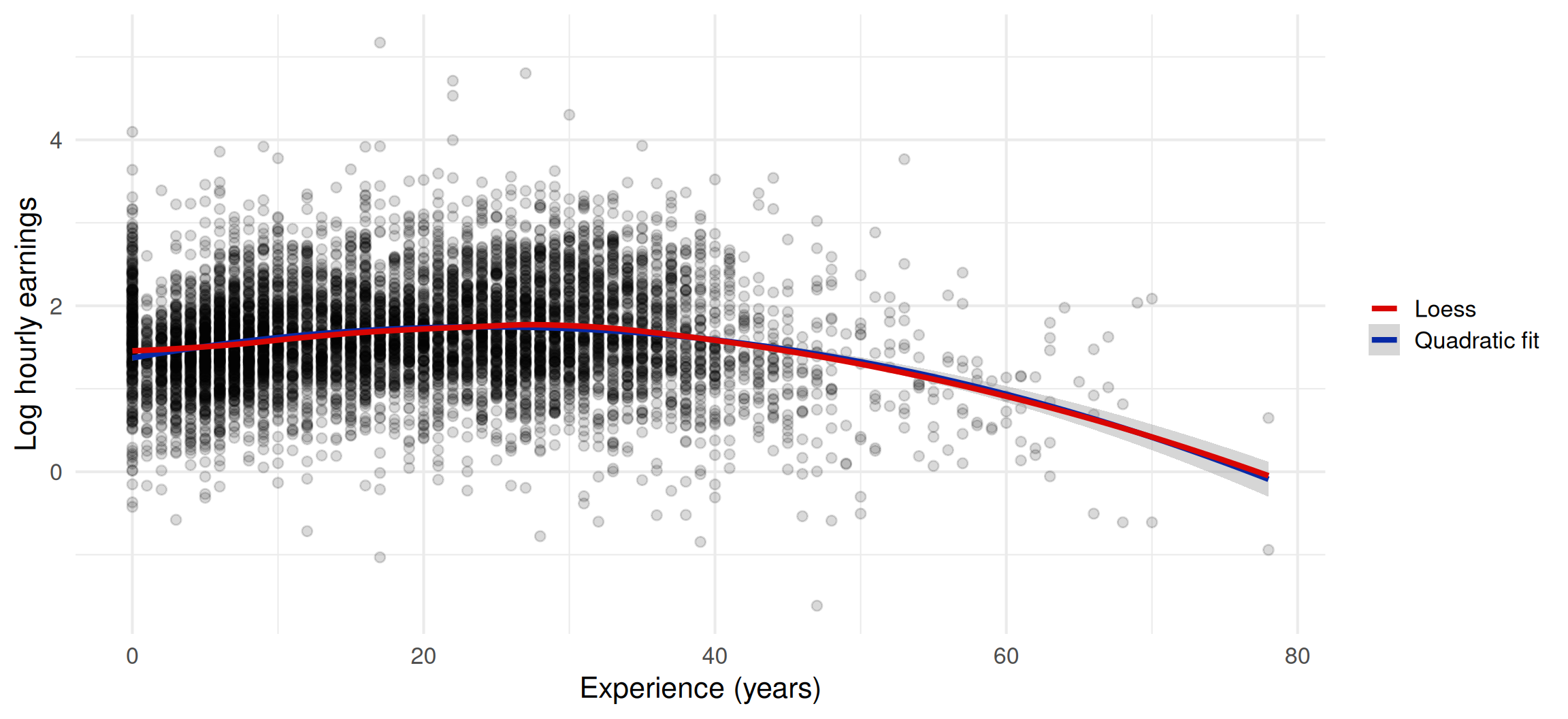
  • \(\hat\beta_2 > 0\) and \(\hat\beta_3 < 0\), both very significant: the experience-earnings profile is concave.
  • Earnings peak at \(-\hat\beta_2 / (2\hat\beta_3) \approx\) 28.6 years of experience.

Exercise #3: the quadratic fit

ggplot(df_w, aes(x = exp, y = lhearnings1def)) +
  geom_point(alpha = 0.15) +
  geom_smooth(aes(colour = "Quadratic fit"), method = "lm",
              formula = y ~ x + I(x^2), se = TRUE) +
  geom_smooth(aes(colour = "Loess"), method = "loess", formula = y ~ x, se = FALSE) +
  scale_colour_manual(name = NULL, values = c("Quadratic fit" = "#0729a6", "Loess" = "#d90502")) +
  labs(x = "Experience (years)", y = "Log hourly earnings") +
  theme_minimal(base_size = 16)

Exercise #3: more covariates

Questions

Try adding a variable indicating whether the individual is a male or a female to the regression. Also try to add variables indicating the number of hours worked in a day by the individual (hoursaday1), and their occupation (occupation1). Discuss the addition of covariates in the model.

Exercise #3: more covariates

gender is equal to 1 for men. occupation1 is an occupation code: the numbers have no meaning, so we include it as a set of dummies with factor().

reg_gender <- lm(lhearnings1def ~ grade + exp + I(exp^2) + gender,
                 data = df_w)

reg_hours  <- lm(lhearnings1def ~ grade + exp + I(exp^2) + gender +
                   hoursaday1,
                 data = df_w)

reg_occ    <- lm(lhearnings1def ~ grade + exp + I(exp^2) + gender +
                   hoursaday1 + factor(occupation1),
                 data = df_w)

Exercise #3: comparing the models

  Model 1 Model 2 Model 3 Model 4 Model 5 Model 6
Years of education 0.065*** 0.071*** 0.070*** 0.070*** 0.068*** 0.035***
  (0.002) (0.002) (0.002) (0.002) (0.002) (0.002)
Experience   0.007*** 0.034*** 0.032*** 0.034*** 0.030***
    (0.001) (0.002) (0.002) (0.002) (0.001)
Experience squared     -0.001*** -0.001*** -0.001*** -0.001***
      (0.000) (0.000) (0.000) (0.000)
Male       0.145*** 0.153*** 0.175***
        (0.014) (0.013) (0.013)
Hours worked per day         -0.073*** -0.069***
          (0.005) (0.004)
Constant 1.070*** 0.871*** 0.695*** 0.621*** 1.210*** 2.006***
  (0.018) (0.023) (0.025) (0.026) (0.046) (0.080)
Occupation dummies No No No No No Yes
R2 0.130 0.151 0.189 0.202 0.228 0.360
Adj. R2 0.130 0.151 0.189 0.202 0.227 0.357
Num. obs. 7091 7091 7091 7091 7091 7091
***p < 0.01; **p < 0.05; *p < 0.1

Exercise #3: discussion

  • Gender is a good control: it is determined before education. Men earn about 16% more than women with the same education and experience. The return to education does not change because, among wage earners, men and women have similar education.
  • Hours worked and occupation are bad controls: they are themselves outcomes of education. With occupation dummies, we compare workers in the same occupation: we shut down one of the main channels through which education raises earnings, and the coefficient is divided by two (0.07 \(\rightarrow\) 0.035).
  • The negative coefficient on hours is partly mechanical: the outcome is earnings per hour, so hours are on both sides of the equation.

More on bad controls

Exercise #3: which model?

  • A higher \(R^2\) does not make a better model for our question: the model with occupation dummies explains earnings better, but it does not estimate the causal effect of education.
  • For the effect of education, our preferred model is column 4: years of education, experience, experience squared and gender.
  • Even this model is not causal: ability, motivation and family background are still omitted. To estimate the causal effect of education, we need variation in education that is unrelated to these factors, e.g. a school construction program (Duflo 2001).

Additional slides

The restricted value-added model

Finally, Andrabi et al. (2011) estimate a model which they call a restricted model:

\[y_{it} - y_{it-1} = \alpha_0 + \alpha_1 P_{it} + u_{it}\]

Dependent variable: English test score (Andrabi et al. 2011)
Model (key assumption, estimator) Persistence Private school
M1. Restricted value-added (perfect persistence \(\beta = 1\), OLS) 1.00 \(-0.08\) (0.02)
M2. Lagged value-added (no effects, no measurement error, OLS) 0.52 (0.02) 0.31 (0.02)

Questions

In what way is it restricted? What do the results suggest?

The restricted value-added model

  • It is restricted in the sense that the effect of prior test scores on current test scores is assumed to be one (\(\beta = 1\), perfect persistence): rewrite the lagged model with \(\beta = 1\).
  • If we assume \(\beta = 1\), private schools have no effect (\(-0.08\)).
  • But when \(\beta\) is estimated, there is only partial persistence (\(\hat\beta = 0.52\)): children who were good in English partly forget and slump back, and children who were bad catch up.
  • In that model, private schools do increase test scores (0.31): they select better students to start with, but they also help them keep their advantage.

Back

The omitted variable bias formula

Let the long regression be \(Y_i = \beta_0 + \beta_1 Educ_i + \beta_2 Exp_i + \varepsilon_i\) and the short regression \(Y_i = b_0 + b_1 Educ_i + e_i\). Then:

\[b_1 = \beta_1 + \beta_2 \times \delta_1\]

where \(\delta_1\) is the coefficient of the regression of the omitted variable on education: \(Exp_i = \delta_0 + \delta_1 Educ_i + u_i\).

short <- lm(lhearnings1def ~ grade, data = df_w)
long  <- lm(lhearnings1def ~ grade + exp, data = df_w)
aux   <- lm(exp ~ grade, data = df_w)

coef(short)["grade"]
     grade 
0.06450398 
coef(long)["grade"] + coef(long)["exp"] * coef(aux)["grade"]
     grade 
0.06450398 

\(\beta_2 > 0\) and \(\delta_1 < 0\): the bias \(\beta_2 \times \delta_1\) is negative, the short regression underestimates \(\beta_1\).

Back

Bad controls

Bad control

A bad control is a variable that is itself an outcome of the treatment. Good controls are variables fixed (determined) before the treatment (Angrist and Pischke 2009, sec. 3.2.3).

  • Education \(\rightarrow\) occupation \(\rightarrow\) earnings: part of the effect of education goes through occupation (graduates become engineers or civil servants rather than farm workers).
  • Controlling for occupation compares a graduate and a non-graduate who are both, say, clerks. This is not the effect of education: the graduate who ended up as a clerk is probably not a typical graduate (selection).
  • The same reasoning applies to hours worked, and in general to any variable measured after the treatment, as in the balance table of Tutorial 2.

Back

References

Andrabi, Tahir, Jishnu Das, Asim Ijaz Khwaja, and Tristan Zajonc. 2011. “Do Value-Added Estimates Add Value? Accounting for Learning Dynamics.” American Economic Journal: Applied Economics 3 (3): 29–54. https://doi.org/10.1257/app.3.3.29.
Angrist, Joshua D., and Jörn-Steffen Pischke. 2009. Mostly Harmless Econometrics: An Empiricist’s Companion. Princeton University Press.
Card, David, and Alan B. Krueger. 1994. “Minimum Wages and Employment: A Case Study of the Fast-Food Industry in New Jersey and Pennsylvania.” American Economic Review 84 (4): 772–93.
Duflo, Esther. 2001. “Schooling and Labor Market Consequences of School Construction in Indonesia: Evidence from an Unusual Policy Experiment.” American Economic Review 91 (4): 795–813.
Imbert, Clément. 2013. “Decomposing the Labor Market Earnings Inequality: The Public and Private Sectors in Vietnam, 19932006.” The World Bank Economic Review 27 (1): 55–79. https://doi.org/10.1093/wber/lhs009.
Mincer, Jacob. 1974. Schooling, Experience, and Earnings. National Bureau of Economic Research.