Math Camp

Session 1: Foundamentals in calculus for economists

Alexandre Grellet

2026-07-30

Getting to know each other

• Who are you?
• What is your academic background?
• Why did you choose the master’s in economics?
• Give 1 (non-academic) hobby.

The purpose is that you get to know each other. That’s also the role of the pre-semester week!

Why study mathematics?

A very central place in economics

• Econometrics (limits, convergence, linear algebra, matrices, etc.)
• Microeconomics (optimization, convex analysis, differentiation, Bayesian probabilities, etc.)
• Macroeconomics (optimal control, Bellman equations, log-linearization, etc.)

This course

Objective: study core concepts in mathematics. We will not have time to cover everything you will see during the master’s, but the class should help you practice with the most important tools and provide you with resources to know where to find relevant information in the next 2 years.

Structure: 1.5 weeks of teaching (24h) + additional hours across the semester (office hours). During this first week, we will have lectures in the morning and practice sessions in the afternoon. Total: 12h of lectures, 12h of tutorials.

Method: In the lectures, we will introduce the concepts and results and apply them in examples. You will prepare exercises for the practice sessions, which we then discuss together.

Core resources

• 3Blue1Brown: essence of calculus and linear algebra series.
• Simon and Blume (1994); Sydsaeter et al. (2021)
• Cummings (2021) and its companion website.

The program

• Session 1: Foundations, sequences, and linearity ← you are here
• Session 2: Linear algebra and OLS
• Session 3: Integration
• Session 4: Compactness, convexity and optimization I
• Session 5: Compactness, convexity and optimization II

Today’s roadmap

1. Continuity: what it means for functions to behave nicely
2. Sequences: the language of limits and convergence
3. Rates of convergence: making “close” precise with big-O and little-o notations
4. Linearization: MVT, Taylor, Jacobians, and the implicit function theorem

The thread running through everything: nonlinear problems can be studied locally through linear approximations. Continuity and sequences are the tools that make that idea rigorous.

Part 0: Sequences

Do you need a review of basic properties?

• If we do not review it but you would need it, you might be lost later on.
• If we review it while you don’t need it, I will be less precise on other material.

I am accountable for the trade-off, but you need to state your true preferences.

Why sequences?

Sequences are ubiquitous in mathematical analysis. Virtually every limit, every notion of convergence, and every continuity argument can be expressed as a statement about sequences.

Later in the master’s, sequences will reappear constantly in statistics and econometrics: estimators are sequences indexed by sample size, and the central question is whether they converge, and how fast.

You may check more complete ressources on sequences. For instance, chapter 9 in Cummings (2021)

Sequences: definition and notation

Definition: Sequence

A sequence in \(\mathbb{R}\) is a function \(a: \mathbb{N} \to \mathbb{R}\). We write it as \((a_n)_{n \geq 1}\) or simply \((a_n)\).

Examples:

• \(a_n = \frac{1}{n}\): the sequence \(1,\, \frac{1}{2},\, \frac{1}{3},\, \frac{1}{4},\, \ldots\)
• \(a_n = (-1)^n\): the sequence \(-1,\, 1,\, -1,\, 1,\, \ldots\)
• \(a_n = \left(1 + \frac{1}{n}\right)^n\): famous because it converges to \(e \approx 2.718\ldots\)

Sequences vs. sets

\((a_n)\) is ordered and allows repetition. The sequence \(1,\, 1,\, 1,\, \ldots\) is perfectly valid. Order matters: \((1, 2, 3, \ldots) \neq (2, 1, 3, \ldots)\) as sequences.

Convergence: the formal definition

Definition: Convergence

A sequence \((a_n)\) converges to a limit \(L \in \mathbb{R}\), written \(a_n \to L\) or \(\lim_{n\to\infty} a_n = L\), if:

\[\forall \varepsilon > 0,\; \exists N \in \mathbb{N} : n > N \implies |a_n - L| < \varepsilon\]

In words: no matter how small a tolerance \(\varepsilon\) you demand, eventually all terms of the sequence fall within that tolerance of \(L\).

A sequence that does not converge to any finite limit is called divergent.

Unpacking the quantifiers as if it was a game:

• \(\forall \varepsilon > 0\): the other player picks any positive tolerance, however tiny.
• \(\exists N\): you get to choose a threshold, which may depend on \(\varepsilon\).
• \(n > N \implies |a_n - L| < \varepsilon\): after your threshold, you win every round (all values are within the limit and the limit + tolerance \(L+\varepsilon\)).

Convergence: intuition

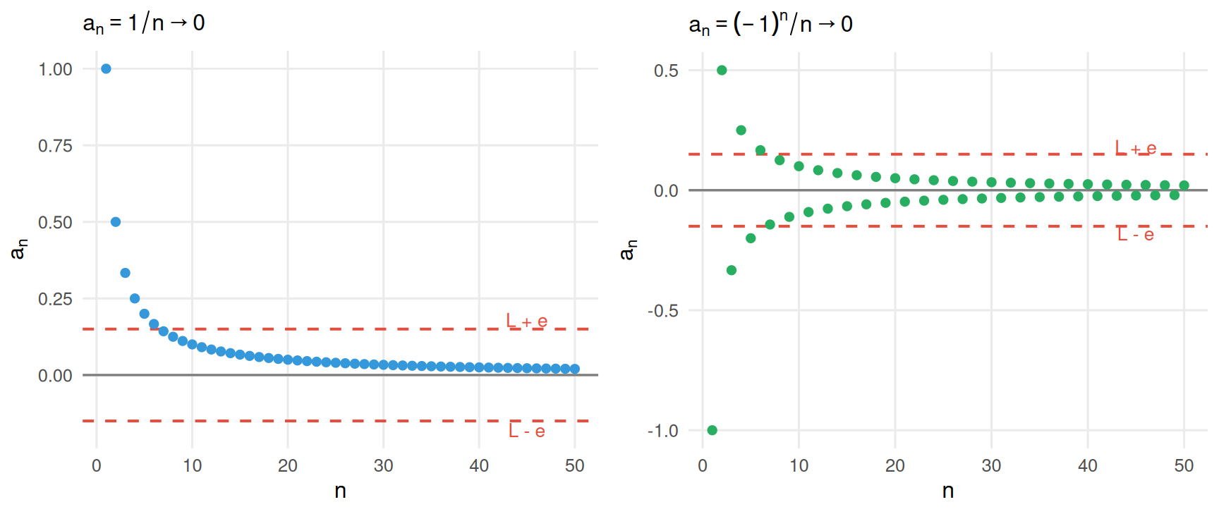
Both sequences converge to 0: one monotonically, one by oscillating. The \(\varepsilon\)-band makes convergence visible: past some threshold \(N\), every term stays inside it.

Sequences and continuity: the connection

We can now state precisely what the sequential definition of continuity means:

Proposition

\(f\) is continuous at \(x\) if and only if for every sequence \((x_n)\) with \(x_n \to x\), we have \(f(x_n) \to f(x)\).

This is not just another formulation. It is often the most useful one in practice: to check continuity, you check whether the function commutes with limits. To disprove continuity, you exhibit one sequence that fails.

🧠 Quick check: convergence

True or False? Discuss with a neighbor (1 minute each).

1. If \(|a_n| \to 0\), then \(a_n \to 0\).
2. If \(a_n \to L\) and \(a_n \to M\), then \(L = M\) (limits are unique).
3. If \(a_n \to L\), then \(a_{2n} \to L\).
4. If \(a_{2n} \to L\) and \(a_{2n+1} \to L\), then \(a_n \to L\).

Answers

1. True. \(|a_n| \to 0 \iff a_n \to 0\) directly from the definition.
2. True. Pick \(\varepsilon < |L-M|/2\). The two \(\varepsilon\)-balls around \(L\) and \(M\) are disjoint, but \((a_n)\) cannot eventually land in both.
3. True. A subsequence of a convergent sequence converges to the same limit.
4. True. Every term is eventually within \(\varepsilon\) of \(L\) via one of the two subsequences, and together they cover all indices.

Algebra of limits

Theorem: Algebra of Limits

If \(a_n \to L\) and \(b_n \to M\) (both finite), then:

• \(a_n + b_n \to L + M\)
• \(\lambda\, a_n \to \lambda L\) for any scalar \(\lambda \in \mathbb{R}\)
• \(a_n \cdot b_n \to L \cdot M\)
• \(\dfrac{a_n}{b_n} \to \dfrac{L}{M}\) provided \(M \neq 0\) and \(b_n \neq 0\) eventually
• If \(a_n \leq b_n\) for all \(n\), then \(L \leq M\) (order is preserved at the limit)

These rules are used constantly. Every time you compute a limit by breaking it into simpler pieces, you are applying this theorem.

Cauchy sequences and completeness

Definition: Cauchy Sequence

\((a_n)\) is Cauchy if its terms eventually become arbitrarily close to each other:

\[\forall \varepsilon > 0,\; \exists N : m, n > N \implies |a_m - a_n| < \varepsilon\]

Theorem: Completeness of \(\mathbb{R}\)

In \(\mathbb{R}\): a sequence converges if and only if it is Cauchy.

Why this is useful. To verify convergence via the definition, you need to know the limit in advance. With Cauchy, you only need to check that terms bunch together. This is often much easier.

Subsequences and Bolzano-Weierstrass

Definition: Subsequence

A subsequence of \((a_n)\) is a sequence \((a_{n_k})_{k \geq 1}\) where \(n_1 < n_2 < n_3 < \cdots\) is a strictly increasing sequence of indices.

Theorem: Bolzano-Weierstrass

Every bounded sequence in \(\mathbb{R}\) has a convergent subsequence.

This is not obvious. The sequence \(((-1)^n)\) oscillates and never converges, yet it has two convergent subsequences: \((1, 1, 1, \ldots)\) and \((-1, -1, -1, \ldots)\).

Economic relevance

Bolzano-Weierstrass underpins existence proofs. When you need to extract a convergent subsequence from a sequence of strategies, prices, or allocations, this theorem does the work. It reappears in the proof of the extreme value theorem.

Monotone convergence theorem

Theorem: Monotone Convergence

• A sequence that is increasing (\(a_{n+1} \geq a_n\)) and bounded above converges.
• A sequence that is decreasing (\(a_{n+1} \leq a_n\)) and bounded below converges.

This is one of the most practically useful results in the course. To show convergence, you just need two things:

1. The sequence is monotone (check the sign of \(a_{n+1} - a_n\))
2. The sequence is bounded (find a ceiling or a floor)

No need to know the limit in advance.

Example: value function iteration

In dynamic programming, the iteration \(V_{n+1}(x) = \max_a [r(x,a) + \delta V_n(x')]\) produces a sequence \((V_n)\). Under standard conditions this sequence is monotone and bounded, so it converges to the true value function \(V^*\). The monotone convergence theorem is at the core of that proof.

Part I: Continuity

Continuity: multiple views

Can you propose definitions for continuity of a function in \(\mathbb{R}\)?

Continuity

The following are definitions of continuity:

• The limit \(\lim_{h\rightarrow0}f(x+h)=f(x)\).
• \(\forall x \in \mathbb{R}\,\forall\epsilon>0\,\exists\delta>0\, \forall y \in \mathbb{R}:\,\|x-y\|<\delta\implies \|f(x)-f(y)\|<\epsilon\)
• Preimage of an open set is also an open set.
• In terms of sequences: \(x_n\rightarrow_{n\to+\infty} x\implies f(x_n)\rightarrow_{n\to+\infty} f(x)\).

Continuity vs uniform continuity

We use the following definition of continuity:

\[\forall x \in \mathbb{R}\,\forall\epsilon>0\,\exists\delta>0\, \forall y \in \mathbb{R}:\,\|x-y\|<\delta\implies \|f(x)-f(y)\|<\epsilon\]

There exists a stronger version of continuity:

Definition: Uniform continuity

A function is uniformly continuous if

\[\forall\epsilon>0\,\exists\delta>0\:\,\forall x,y \in \mathbb{R}\, \|x-y\|<\delta\implies \|f(x)-f(y)\|<\epsilon\]

Can you state the main difference? Dos one imply the other?

🧠 Short exercise: uniform vs. pointwise

Two minutes. Discuss with your neighbor:

Consider \(f(x) = x^2\) on \(\mathbb{R}\).

1. Is \(f\) continuous on \(\mathbb{R}\)? (Use the \(\varepsilon\)-\(\delta\) definition.)
2. Is \(f\) uniformly continuous on \(\mathbb{R}\)? Try to find a counterexample — pick any \(\varepsilon\) and argue that no single \(\delta\) works for all \(x\).
3. Is \(f\) uniformly continuous on \([0, 10]\)? Why?

Key Intuition

The difference is whether \(\delta\) can depend on \(x\) (continuity) or must work simultaneously for all \(x\) (uniform continuity). On \(\mathbb{R}\), the slope of \(x^2\) grows without bound: so you need a smaller and smaller \(\delta\) as \(x\) gets large (i.e. for two numbers with equal distance, the necessary \(\delta\) is not the same depending on how large the numbers are).

Two sketches of proof:

• By contradiction. Assume that uniform continuity holds. Then for some \(\delta\) given a specific \(\epsilon\), we have \(|x−y|<\delta\Rightarrow |f(x)−f(y)|=|x^2−y^2|<\varepsilon\). Use that \(|x^2−y^2| = |x−y||x+y|\) to prove a contradiction. In this case, it’s that you need: \(|x+y|<\frac{\varepsilon}{\delta}\). But for any \(\delta\), you will be able to find some \(x,y\) that contradict this while having \(|x−y|<\delta\)
• By counter-example: take sequences \(u_n\equiv n^2+\frac1n,v_n\equiv n^2\).

Compact and complete sets

Definition: Compact Set

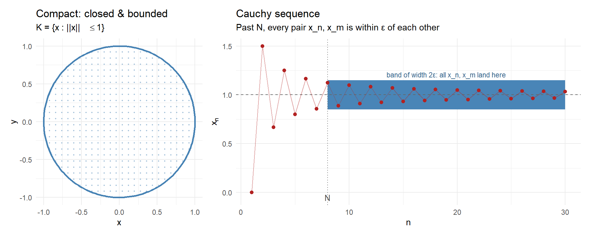
A set \(K \subset \mathbb{R}^n\) is compact if every open cover of \(K\) has a finite subcover. In \(\mathbb{R}^n\), this is equivalent (by the Heine-Borel theorem) to \(K\) being closed and bounded.

Definition: Complete Metric Space

A metric space \((X, d)\) is complete if every Cauchy sequence in \(X\) converges to a limit that is also in \(X\). Recall: \(\{x_n\}\) is Cauchy if \(\forall \varepsilon > 0,\, \exists N : m,n > N \Rightarrow d(x_m, x_n) < \varepsilon\).

Examples and non-examples:

Set	Compact?	Complete?
\([0,1] \subset \mathbb{R}\)	✅ closed & bounded	✅ closed subset of \(\mathbb{R}\)
\((0,1) \subset \mathbb{R}\)	❌ not closed	❌ sequence \(1/n\) is Cauchy, limit \(0 \notin (0,1)\)
\(\mathbb{R}\)	❌ not bounded	✅ every Cauchy sequence converges
\(\mathbb{Q}\)	❌ neither	❌ \(3, 3.1, 3.14, 3.141, \ldots \to \pi \notin \mathbb{Q}\)
\(\{x \in \mathbb{R}^2 : \|x\| \leq 1\}\)	✅ closed ball	✅

Why economists care

Compact action sets guarantee that optimization problems have a solution (Weierstrass extreme value theorem - will study it later on). Completeness underlies fixed-point theorems (Banach, Brouwer) used to prove equilibrium existence in game theory and general equilibrium.

Illustrations

Continuous on compact \(\Rightarrow\) uniformly continuous (I)

Theorem (Heine–Cantor)

If \(f: K \to \mathbb{R}\) is continuous on a compact set \(K\subset\mathbb{R}\), then \(f\) is uniformly continuous on \(K\).

Proof

Let \(\varepsilon > 0\). For each \(x\in K\), continuity at \(x\) gives \(\delta_x>0\) such that

\[|f(x) - f(y)| < \varepsilon \quad\text{whenever}\quad |x - y| < \delta_x.\]

The collection of open intervals \(\{(x - \tfrac{\delta_x}{2},\, x + \tfrac{\delta_x}{2}) : x\in K\}\) covers \(K\). By compactness, choose a finite subcover

\[K \;\subset\; \bigcup_{i=1}^n \Bigl(x_i - \tfrac{\delta_{x_i}}{2},\,x_i + \tfrac{\delta_{x_i}}{2}\Bigr).\]

Let \(\delta = \min_{1\le i\le n} \delta_{x_i}/2 > 0\).

Then for any \(x,y\in K\) with \(|x-y|<\delta\), there is some \(i\) so that \(x\) and \(y\) both lie in \(\bigl(x_i - \tfrac{\delta_{x_i}}{2},\,x_i + \tfrac{\delta_{x_i}}{2}\bigr)\).

Hence \(|f(x) - f(y)| < \varepsilon\), showing uniform continuity. \(\blacksquare\)

Economic Relevance

Why does this matter in economics? When we model agents acting on a bounded price or income space (a compact set), well-behaved utility functions are automatically uniformly continuous \(\rightarrow\) small changes in prices lead to small, controlled, changes in demand. The unbounded case (\(\mathbb{R}\)) is trickier, which is one reason we often impose boundedness assumptions in theory.

Part II: Rates of Convergence

Why rates matter

Knowing that a sequence converges is useful. Knowing how fast it converges is often what you actually need.

Consider two sequences that both converge to zero:

\[a_n = \frac{1}{n} \qquad \text{and} \qquad b_n = \frac{1}{n^{100}}\]

They converge to the same limit, but \(b_n\) reaches zero vastly faster. In analysis, in numerical methods, and in statistics, the rate of convergence determines what you can conclude. We need precise language for this.

Little-o notation

Definition: Little-\(o\)

We say \(f(x) = o(g(x))\) as \(x \to x_0\) if:

\[\lim_{x \to x_0} \frac{f(x)}{g(x)} = 0\]

In words: \(f\) is negligible relative to \(g\) near \(x_0\).

Key examples as \(x \to 0\):

Statement	True?	Why
\(x^2 = o(x)\)	✅	\(x^2/x = x \to 0\)
\(x = o(x^2)\)	❌	\(x/x^2 = 1/x \to \infty\)
\(e^x - 1 - x = o(x)\)	✅	the remainder is quadratic
\(e^x - 1 - x = o(x^2)\)	❌	\((e^x-1-x)/x^2 \to 1/2 \neq 0\)

The last row will be crucial when we study Taylor approximations.

Big-O notation

Definition: Big-\(O\)

We say \(f(x) = O(g(x))\) as \(x \to x_0\) if there exist constants \(C > 0\) and \(\delta > 0\) such that:

\[|x - x_0| < \delta \implies |f(x)| \leq C\,|g(x)|\]

In words: \(f\) is bounded in magnitude relative to \(g\) near \(x_0\). We say \(f\) is at most of order \(g\).

For sequences

\((a_n) = O(b_n)\) if \(\exists\, C > 0\) and \(N\) such that \(n > N \implies |a_n| \leq C|b_n|\).

\((a_n) = o(b_n)\) if \(a_n / b_n \to 0\).

Key relationship: \(o(g)\) implies \(O(g)\), but not the other way around. A sequence that is \(o(b_n)\) goes to zero even after scaling by \(b_n^{-1}\); a sequence that is merely \(O(b_n)\) stays bounded after that scaling.

🧠 Exercise: big-O vs. little-o

Solo (2 minutes), then compare with a neighbor.

Classify each as \(O(n^{-1/2})\), \(o(n^{-1/2})\), or neither, as \(n\to\infty\):

1. \(a_n = \dfrac{1}{\sqrt{n}}\)
2. \(a_n = \dfrac{\ln n}{\sqrt{n}}\)
3. \(a_n = \dfrac{1}{n}\)
4. \(a_n = \dfrac{1}{n^{1/3}}\)

Answers

1. \(O(n^{-1/2})\): ratio equals 1, so bounded. Not \(o(n^{-1/2})\).
2. Neither: \(a_n / n^{-1/2} = \ln n \to \infty\), so \(a_n\) is actually larger than \(n^{-1/2}\) asymptotically. A good trap.
3. \(o(n^{-1/2})\): \(\frac{1/n}{1/\sqrt{n}} = \frac{1}{\sqrt{n}} \to 0\). Also \(O(n^{-1/2})\).
4. Neither: \(\frac{n^{-1/3}}{n^{-1/2}} = n^{1/6} \to \infty\).

Part III: Linearization

Linearity: can you guess why it’s central?

A. Linear models can capture any non-linear relationship exactly.

B. Linear functions are easy to estimate and interpret.

C. Any sufficiently smooth function can be locally approximated by a linear one.

D. The consumer’s budget set is always represented by a linear constraint.

E. Linear operators enjoy the superposition principle.

F. Numerical algorithms (OLS, QR decomposition) rely on linear algebra.

→ In practice, mainly B and C. This is why linear algebra and calculus are non-negotiable.

Mean value theorem

Mean value theorem (in \(\mathbb{R}\))

Theorem

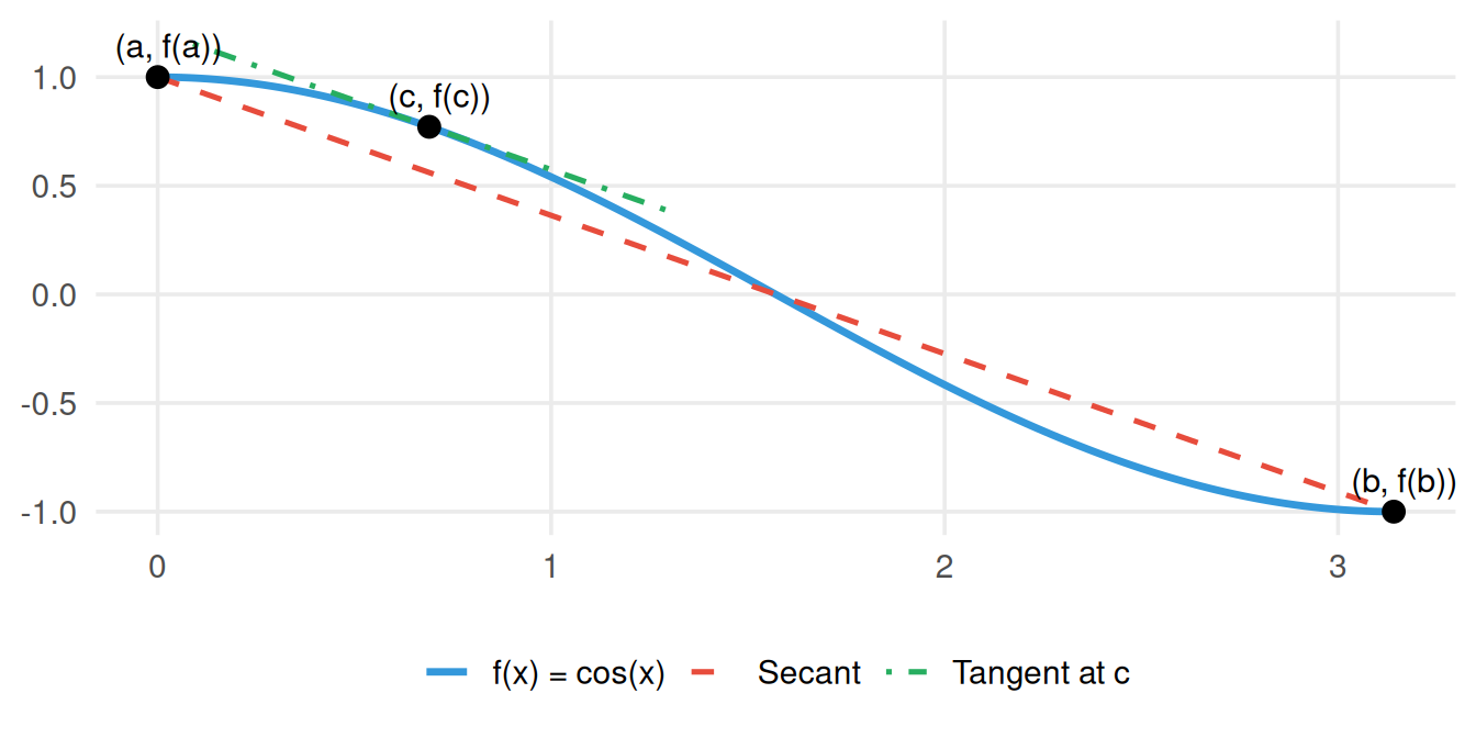
If \(f\) is continuous on \([a,b]\) and differentiable on \((a,b)\), then \[\exists c \in (a,b): f(b)-f(a)=(b-a)f'(c)\]

Usefulness of MVT

Why do you think MVT is useful?

• It gives a relationship between average and marginal changes. You can formulate it as: “for any smooth production plan \(Q(p)\) defined on \(x\in [a,b]\), there exists a price \(p^*\in (a,b)\) such that: \[\frac{Q(b)-Q(a)}{b-a}=Q'(p^*)\]
• It provides a first basis for linear approximations: \[f(a+\varepsilon)-f(a)\sim \varepsilon f'(a)\] since \(c\) cannot be far away from \(a\) if \(\varepsilon\) is small;
• It will be useful to introduce more important results later on.

🧠 Quick check: true or false?

Discuss with a neighbor (1 minute each):

1. True or False: If \(f\) is differentiable and \(f'(x)=0\) for all \(x\in(a,b)\), then \(f\) is constant on \([a,b]\). (Use MVT to prove or disprove!)

2. True or False: If \(f(a)=f(b)\), then \(\exists\, c\in(a,b)\) with \(f'(c)=0\).

1. Easy to prove using that you can pick any \(c\) and MVT.
2. Special case of MVT called Rolle’s theorem.

Taylor’s theorem

Taylor’s Theorem

Taylor’s Theorem (Lagrange remainder)

Let \(I \subset \mathbb{R}\) be an open interval containing \(a\), and let \(f \in \mathcal{C}^{n+1}(I)\). The Taylor polynomial of degree \(n\) for \(f\) about \(a\) is \[ P_n(x) \;=\; \sum_{k=0}^{n} \frac{f^{(k)}(a)}{k!}\,(x - a)^k . \] Then for every \(x \in I\) there exists \(\xi\) strictly between \(a\) and \(x\) such that \[ f(x) \;=\; P_n(x) + \frac{f^{(n+1)}(\xi)}{(n+1)!}\,(x-a)^{n+1}. \]

Weaker version. If \(f\) is only \(\mathcal{C}^n\), one still gets the qualitative (Peano) form \(f(x) = P_n(x) + o\big((x-a)^n\big)\) as \(x \to a\) — it pins down the order of the error but not its exact size.

Local approximation. Writing \(x = a+\varepsilon\), \[ f(a+\varepsilon) \;=\; \underbrace{\sum_{k=0}^{n} \frac{f^{(k)}(a)}{k!}\,\varepsilon^k}_{P_n(a+\varepsilon)} \;+\; \underbrace{O(\varepsilon^{n+1})}_{\text{remainder}}. \]

📝 Worked example: approximating utility

Setup. A consumer has CRRA utility \(U(c) = \frac{c^{1-\sigma}-1}{1-\sigma}\), where:

• \(c > 0\) is consumption, \(\sigma > 0\), \(\sigma \neq 1\)
• \(\sigma\) is the coefficient of relative risk aversion: \(\sigma = -\frac{U''(c)\,c}{U'(c)}\)
• We expand around \(c^* = 1\) (a normalization)

Compute derivatives at \(c^*=1\):

\[U'(c) = c^{-\sigma} \Rightarrow U'(1) = 1 \qquad U''(c) = -\sigma c^{-\sigma-1} \Rightarrow U''(1) = -\sigma\]

Degree-2 Taylor approximation:

\[U(c) \approx \underbrace{(c-1)}_{\text{linear gain}} - \underbrace{\frac{\sigma}{2}(c-1)^2}_{\text{curvature penalty}}\]

Interpretation

Consider a lottery: consumption is either \(1+\varepsilon\) or \(1-\varepsilon\) with equal probability. Expected utility is:

\[\mathbb{E}[U(c)] \approx \left(0\right) - \frac{\sigma}{2}\varepsilon^2\]

The linear terms cancel by symmetry. What remains is \(-\frac{\sigma}{2}\varepsilon^2 < 0\): the consumer strictly prefers \(c=1\) for sure. The larger \(\sigma\), the bigger the penalty. In this regard, why is CRRA utility attractive?

📝 Worked example: log-linearization

The problem. \(f(x) = \ln x\) is nonlinear — but economists work with it constantly (utility, production, prices). Can we linearize it usefully?

Taylor around \(x^* > 0\):

\[\ln x \approx \ln x^* + \frac{1}{x^*}(x - x^*) = \ln x^* + \frac{x - x^*}{x^*}\]

So for \(x\) close to \(x^*\), the log-deviation from \(x^*\) satisfies:

\[\ln x - \ln x^* \approx \frac{x - x^*}{x^*}\]

In words: a log-difference is approximately a percentage deviation. This is one of the reasons why using logs is so ubiquitous.

This approach is quite important in macroeonomics and you will use it a lot. See some notes by Eric Sims.

🧠 Exercise: Taylor expand key economic functions

Solo (3 minutes), then compare with a neighbor.

Find the second-order Taylor expansion around the indicated point:

1. \(f(x) = \ln(1+x)\) around \(x=0\).

2. \(f(r) = \frac{1}{(1+r)^T}\) (present-value factor) around \(r=0\). (Hint: what does the approximation tell you about small interest rate changes?)

3. \(f(x) = e^x\) around \(x=0\).

Answers

1. \(\ln(1+x) \approx x - \frac{x^2}{2}\)

2. \(\frac{1}{(1+r)^T} \approx 1 - Tr + \frac{T(T+1)}{2}r^2\)

3. \(e^x \approx 1 + x + \frac{x^2}{2}\)

For (2): the linear approximation \(1-Tr\) says the present value falls linearly in the interest rate, at rate \(T\) (duration!). The quadratic term captures convexity \(\Rightarrow\) “convexity adjustment.”

Multivariate calculus

Motivation

Most of the time = interested in multiple variables, not a single \(x\).

Goal: Generalize everything we already know in \(\mathbb{R}\) to \(\mathbb{R}^n,\, n\in \mathbb{N}\).

Functions

Functions in \(\mathbb{R}^n\)

A function \(f: \mathbb{R}^n \rightarrow \mathbb{R}^m\) is a mapping that assigns a vector given a vector input.

Example:

• \(f(x,y) = \pmatrix{ x+y\\ x-y\\ x+2y}\)
• \(f(x,y,z) = \pmatrix{ x+y+z\\ x-y}\)
• \(f(x,y) = \pmatrix{ x+y\\ x-y}\)

Continuity in higher dimensions

Just as we defined derivatives in \(\mathbb{R}\) we can define derivatives in higher dimensions. Let \(f: \mathbb{R}^n \mapsto \mathbb{R}^m\).

Continuity

Let \(f: \mathbb{R}^n \mapsto \mathbb{R}^m\), \(x_0\in \mathbb{R}^n\) and \(f(x_0)\) its image. We say that \(f\) is continuous at \(x_0\) if:

• \(\forall \{x_n\}_{n=1}^{+\infty}\in \mathbb{R}^n\) (a sequence) such that \(x_n\rightarrow_{n\rightarrow+\infty}x_0\) we have \(f(x_n)\rightarrow_{n\rightarrow+\infty}f(x_0)\)
• For every open set \(V\subset\mathbb{R}^m\), \(f^{-1}(V)\subset U\) is open in \(\mathbb{R}^n\).
• For every \(\varepsilon>0\) there exists \(\delta>0\) such that \(\|x - x_0\| < \delta \Rightarrow \|f(x) - f(x_0)\| < \varepsilon\)
• If \(f=(f_1,\dots,f_m)\), then \(f\) is continuous at \(x_0\) iff each \(f_i:\mathbb{R}^n\to\mathbb{R}\) is continuous at \(x_0\).

Total derivative

Let \(f: \mathbb{R}^n \mapsto \mathbb{R}\). We refer to the total derivative of \(f\) at \(x_0\) as:

\[df = \frac{\partial f}{\partial x_1}(x_0)dx_1 + \ldots + \frac{\partial f}{\partial x_n}(x_0)dx_n\]

📝 Worked example: total derivative of a cost function

Setup. A firm’s cost function is \(C(w, r, q) = 2\,w^{1/2}\,r^{1/2}\,q\) where \(w\) = wage, \(r\) = rental rate, \(q\) = output.

Total derivative:

\[dC = \frac{\partial C}{\partial w}dw + \frac{\partial C}{\partial r}dr + \frac{\partial C}{\partial q}dq\] \[= w^{-1/2}r^{1/2}q\,dw + w^{1/2}r^{-1/2}q\,dr + 2w^{1/2}r^{1/2}\,dq\]

Interpretation

The total derivative answers: if wages, rents, and output all change simultaneously by small amounts, how much does total cost change?

Each term has a clean meaning:

• \(\frac{\partial C}{\partial w}dw\): the cost increase from a small rise in wages, holding everything else fixed
• \(\frac{\partial C}{\partial r}dr\): same for the rental rate
• \(\frac{\partial C}{\partial q}dq\): the marginal cost — how much more it costs to produce one extra unit

The total effect is just the sum of the individual effects. This is precisely the superposition property of linear approximations.

Continuously differentiable functions

Definition: Continuously Differentiable (\(C^1\))

A function \(f:\mathbb{R}^n\to\mathbb{R}\) is said to be continuously differentiable (or \(C^1\)) on an open set \(U\subset\mathbb{R}^n\) if for each \(i=1,\dots,n\), the partial derivative

\[\frac{\partial f}{\partial x_i}(x)\]

exists for all \(x\in U\) and is continuous in \(x\).

Gradient vector and directional derivative

The gradient of a \(C^1\) function \(f:\mathbb{R}^n\to\mathbb{R}\) at a point \(x^*\) is the vector of partial derivatives:

\[\nabla f(x^*) = \begin{pmatrix} \displaystyle \frac{\partial f}{\partial x_1}(x^*) \\[1ex] \vdots \\[1ex] \displaystyle \frac{\partial f}{\partial x_n}(x^*) \end{pmatrix}\]

The gradient can be used to write the directional derivative in the direction \(v=(v_1,\dots,v_n)\):

\[D f_x(v) \;=\; v\cdot \nabla f(x) \;=\; \sum_{i=1}^n \frac{\partial f}{\partial x_i}(x)\,v_i\]

🧠 Exercise: gradient and indifference curves

Setup. Consider the utility function \(U(x_1, x_2) = x_1^{\alpha} x_2^{1-\alpha}\) with \(\alpha \in (0,1)\).

1. Compute the gradient \(\nabla U\) at a point \((x_1^*, x_2^*)\).
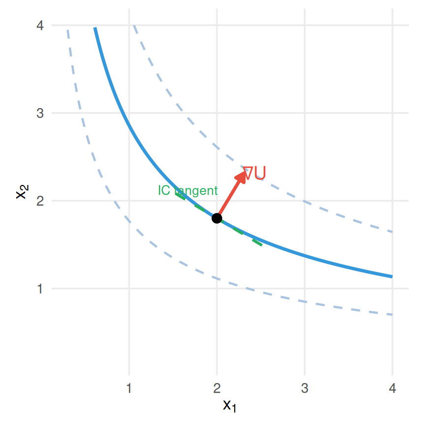
2. The indifference curve at utility level \(\bar{U}\) is defined by \(U(x_1,x_2) = \bar{U}\). What is the direction of \(\nabla U\) relative to the indifference curve?
3. The marginal rate of substitution is \(MRS = -\frac{\partial U/\partial x_1}{\partial U/\partial x_2}\). Compute it and interpret it economically.

Answers

1. \(\nabla U = \bigl(\alpha x_1^{\alpha-1}x_2^{1-\alpha},\; (1-\alpha)x_1^{\alpha}x_2^{-\alpha}\bigr)^\top\)

2. The gradient is orthogonal to the indifference curve. Any direction \(v\) along the curve keeps utility constant, so \(dU = \nabla U \cdot v = 0\). The gradient points away from it, toward higher utility, as steeply as possible.

3. \(MRS = \frac{\alpha\,x_2}{(1-\alpha)\,x_1}\). How many units of \(x_2\) the consumer sacrifices for one more unit of \(x_1\). The indifference curve’s slope is perpendicular to \(\nabla U\) — which is exactly what pins it down.

Jacobian

The gradient of a differentiable function \(F:\mathbb{R}^n\to\mathbb{R}^m\) with components \((f_1, f_2, \ldots, f_m)\) at a point \(x^*\) is the matrix of partial derivatives:

\[J_F(x^*) = \begin{pmatrix} \dfrac{\partial f_1}{\partial x_1}(x^*) & \cdots & \dfrac{\partial f_1}{\partial x_n}(x^*) \\[1ex] \vdots & \ddots & \vdots \\[1ex] \dfrac{\partial f_m}{\partial x_1}(x^*) & \cdots & \dfrac{\partial f_m}{\partial x_n}(x^*) \end{pmatrix}\]

Note that:

\[J_F(x^*) = \begin{pmatrix} \nabla f_1^{\top} \\[1ex] \vdots \\[1ex] \nabla f_m^{\top} \end{pmatrix}\]

📝 Worked example: Jacobian of a demand system

Setup. Suppose demand for two goods depends on their prices:

\[Q_1(p_1, p_2) = 10 - 2p_1 + p_2, \qquad Q_2(p_1, p_2) = 8 + p_1 - 3p_2\]

The Jacobian of \(Q = (Q_1, Q_2)^\top\) with respect to \((p_1, p_2)\) is:

\[J_Q = \begin{pmatrix} \partial Q_1/\partial p_1 & \partial Q_1/\partial p_2 \\ \partial Q_2/\partial p_1 & \partial Q_2/\partial p_2 \end{pmatrix} = \begin{pmatrix} -2 & 1 \\ 1 & -3 \end{pmatrix}\]

Interpretation:

• Diagonal entries = own-price elasticities (in levels): \(\partial Q_1/\partial p_1 = -2\) means raising \(p_1\) by $1 reduces demand for good 1 by 2 units.
• Off-diagonal entries = cross-price effects: goods are substitutes (positive cross-price effects).
• Symmetry of cross-effects is not guaranteed in general.

The chain rule for vector-valued functions

Theorem (Chain Rule)

Let \(F = (f_1,\dots,f_m)\colon \mathbb{R}^n \longrightarrow \mathbb{R}^m\) and \(a\colon \mathbb{R} \longrightarrow \mathbb{R}^n\) be \(C^1\) functions. Then the composite \(g(t) = F\bigl(a(t)\bigr):\mathbb{R}\to\mathbb{R}^m\) is \(C^1\), and for each component \(g_i\):

\[g_i'(t) \;=\; \sum_{j=1}^n \frac{\partial f_i}{\partial x_j}\bigl(a(t)\bigr)\, a_j'(t) \;=\; \nabla f_i\bigl(a(t)\bigr)\;\cdot\;\nabla a(t)\]

Putting these together gives the vector equation:

\[g'(t) \;=\; \nabla\bigl(F\circ a\bigr)(t) \;=\; J_F\bigl(a(t)\bigr)\;\times\;\nabla a(t)\]

The chain rule: comparative statics along a path

Suppose a firm’s profit is a function of prices and wages \(\pi(p, w)\) and both depend on a policy parameter \(t\) (say, a tax). How does profit change with \(t\)?

\[\frac{d\pi}{dt} = \frac{\partial \pi}{\partial p}\frac{dp}{dt} + \frac{\partial \pi}{\partial w}\frac{dw}{dt}\]

The chain rule decomposes the total effect into: the direct effect through prices, plus the direct effect through wages.

MVT in \(\mathbb{R}^n\)

Theorem (Mean Value Theorem in \(\mathbb{R}^n\))

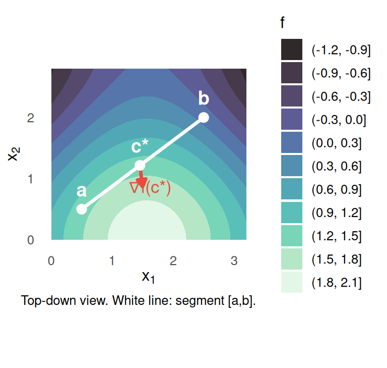
Let \(U\subset\mathbb{R}^n\) be open and convex, and let \(f:U\to\mathbb{R}\) be differentiable. For any \(\mathbf{a},\mathbf{b}\in U\), there exists \(\mathbf{c}\) on the line segment \([\mathbf{a},\mathbf{b}]\) such that \[f(\mathbf{b}) - f(\mathbf{a}) = \nabla f(\mathbf{c}) \cdot (\mathbf{b}-\mathbf{a})\]

Demonstration trick

Interestingly, once you notice that the set is convex, the demonstration of the MVT in \(\mathbb{R}^n\) is very simple. You just use MVT in \(\mathbb{R}\) for the following function:

\[g(t) = f(\mathbf{x} + t(\mathbf{y} - \mathbf{x})) \quad \text{for } t \in [0, 1]\]

🧠 Discussion: why convexity?

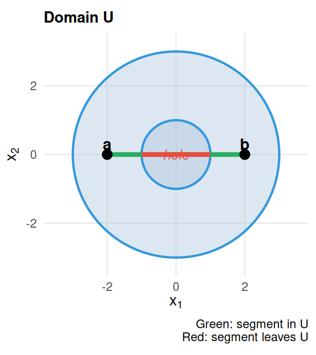
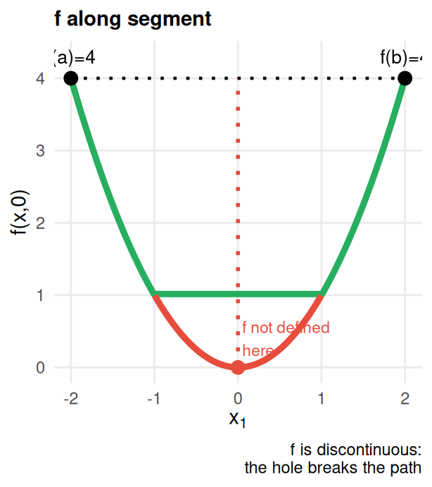
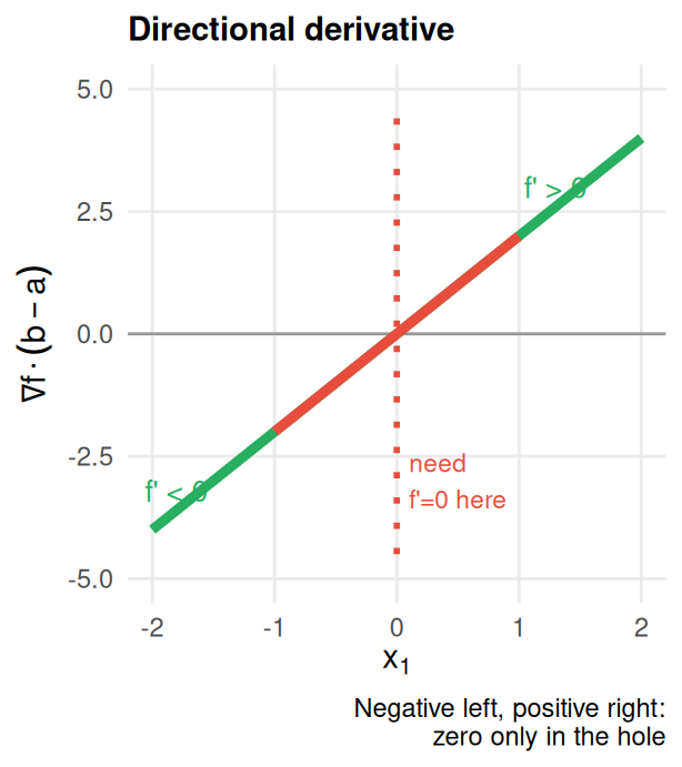
Let \(U\) be a donut \(\{(x,y) : 1 \leq x^2+y^2 \leq 9\}\), \(f(x,y) = x^2 - y^2\), \(\mathbf{a} = (-2, 0)\), \(\mathbf{b} = (2, 0)\).

\(f(\mathbf{a}) = f(\mathbf{b}) = 4\) so MVT would need \(\mathbf{c}\) with \(\nabla f(\mathbf{c})\cdot(\mathbf{b}-\mathbf{a}) = 0\), i.e. \(c_x = 0\). That point is in the hole.

Summary

Requiring the function to be well-defined on the segment is not just a simplification, it’s really required.

Taylor’s theorem in \(\mathbb{R}^n\)

Preliminaries

Multi-Index Notation

Let \(\alpha=(\alpha_1,\dots,\alpha_n)\in\mathbb{N}^n\). Then \[|\alpha|=\alpha_1+\cdots+\alpha_n\] For a \(C^k\) function \(f:\mathbb{R}^n\mapsto\mathbb{R}\), we write \[D^\alpha f =\frac{\partial^{|\alpha|}f} {\partial x_1^{\alpha_1}\,\cdots\,\partial x_n^{\alpha_n}}\]

Example. Take \(n=2\) and \(f(x_1,x_2) = x_1^3 x_2^2\).

• \(\alpha = (2,1)\): then \(|\alpha| = 3\) and \[D^\alpha f = \frac{\partial^{3} f}{\partial x_1^{2}\,\partial x_2^{1}} = 12\,x_1 x_2\]
• \(\alpha = (0,0)\): then \(|\alpha| = 0\) and \(D^\alpha f = f\) itself — the zeroth-order derivative is just the function.

The theorem

Theorem (Multivariate Taylor’s Theorem)

Let \(f: \mathbb{R}^n \mapsto \mathbb{R}\) be \(C^k\) at the point \(a \in \mathbb{R}^n\). Then there exist functions \(h_\alpha \colon \mathbb{R}^n \to \mathbb{R}\), \(|\alpha| = k\), such that

\[f(x) =\sum_{|\alpha|\le k} \frac{D^\alpha f(a)}{\alpha!}\,(x - a)^\alpha \;+\; \sum_{|\alpha| = k} h_\alpha(x)\,(x - a)^\alpha\]

and

\[\lim_{x \to a} h_\alpha(x) \;=\; 0 \quad\text{for each multi-index }\alpha\]

Second-order Taylor in \(\mathbb{R}^2\): motivation

In \(\mathbb{R}^1\), the second-order Taylor expansion is: \[f(a + \varepsilon) \approx f(a) + f'(a)\,\varepsilon + \frac{1}{2}f''(a)\,\varepsilon^2\]

In \(\mathbb{R}^2\), we expand \(f(\mathbf{a} + \boldsymbol{\varepsilon})\) where \(\boldsymbol{\varepsilon} = (\varepsilon_1, \varepsilon_2)^\top\). Applying the 1D result along each direction and collecting terms:

\[f(\mathbf{a} + \boldsymbol{\varepsilon}) \approx f(\mathbf{a}) + \underbrace{\frac{\partial f}{\partial x_1}\varepsilon_1 + \frac{\partial f}{\partial x_2}\varepsilon_2}_{\text{first-order: }{\nabla f(\mathbf{a})^\top \boldsymbol{\varepsilon}}} + \frac{1}{2}\underbrace{\left( \frac{\partial^2 f}{\partial x_1^2}\varepsilon_1^2 + 2\frac{\partial^2 f}{\partial x_1 \partial x_2}\varepsilon_1\varepsilon_2 + \frac{\partial^2 f}{\partial x_2^2}\varepsilon_2^2 \right)}_{\text{second-order: all cross and own effects}}\]

The second-order term collects four second derivatives — can we write this compactly?

The Hessian

The second-order term can be written as a quadratic form \(\boldsymbol{\varepsilon}^\top H_f(\mathbf{a})\,\boldsymbol{\varepsilon}\), where:

\[H_f(\mathbf{a}) = \begin{pmatrix} \dfrac{\partial^2 f}{\partial x_1^2} & \dfrac{\partial^2 f}{\partial x_1 \partial x_2} \\[2ex] \dfrac{\partial^2 f}{\partial x_1 \partial x_2} & \dfrac{\partial^2 f}{\partial x_2^2} \end{pmatrix}\]

So the full second-order expansion is:

\[\boxed{f(\mathbf{x}) \approx f(\mathbf{a}) + \nabla f(\mathbf{a})^\top (\mathbf{x}-\mathbf{a}) + \frac{1}{2}(\mathbf{x}-\mathbf{a})^\top H_f(\mathbf{a})\,(\mathbf{x}-\mathbf{a})}\]

Note: \(H_f\) is symmetric (off-diagonal terms are equal) whenever \(f \in C^2\). (should sound familiar given prerequisites)

Approximation by differentials

Suppose \(F = (f_1,\dots,f_m)\colon \mathbb{R}^n \to \mathbb{R}^m\) is \(C^1\), \(x^*=(x^*_1,\dots,x^*_n)\), \(\Delta x=(\Delta x_1,\dots,\Delta x_n)\).

For each component \(f_i\) we have (by first-order Taylor’s approximation):

\[f_i(x^* + \Delta x) - f_i(x^*) \;\approx\; \frac{\partial f_i}{\partial x_1}(x^*)\,\Delta x_1 + \cdots + \frac{\partial f_i}{\partial x_n}(x^*)\,\Delta x_n\]

Overall, combining these in vector/matrix form gives:

\[F(x^* + \Delta x) - F(x^*) \;\approx\; \begin{pmatrix} \dfrac{\partial f_1}{\partial x_1}(x^*) & \cdots & \dfrac{\partial f_1}{\partial x_n}(x^*) \\[1ex] \vdots & \ddots & \vdots \\[1ex] \dfrac{\partial f_m}{\partial x_1}(x^*) & \cdots & \dfrac{\partial f_m}{\partial x_n}(x^*) \end{pmatrix} \begin{pmatrix} \Delta x_1 \\[0.5ex] \vdots \\[0.5ex] \Delta x_n \end{pmatrix}\]

Implicit function theorem

Introduction

Imagine you are a first-year graduate student in econ. You need to choose how much time to allocate to leisure \(l\) and study \(s\), subject to a very hard constraint: you only have \(T=16\)h available per day.

You need to maximize your welfare:

\[\max_{l,s} W(l,s) \text{ s.t. } l+s= T\]

What you can see: if there is a unique solution, then this solution must be defined by exogeneous variable \(T\) and the system of first-order equations (\(F(l,s) = 0\)). The implicit function theorem tells us how the solution would evolve if \(T\) was to change. This helps understanding comparative statics.

Implicit function theorem

Theorem (Implicit Function Theorem)

Let \(f:\mathbb{R}^{n+m}\to\mathbb{R}^m\) be a continuously differentiable function, and let \(\mathbb{R}^{n+m}\) have coordinates \((x,y)\). Fix a point \((x_0,y_0)\) with \(f(x_0,y_0)=0\). If the Jacobian matrix

\[J_{f,y}(x_0,y_0) = \begin{bmatrix} \frac{\partial f_i}{\partial y_j}(x_0,y_0) \end{bmatrix}_{m\times m}\]

is invertible, then there exists an open set \(U\subset\mathbb{R}^n\) containing \(x_0\) and a unique \(C^1\) function \(g:U\to\mathbb{R}^m\) with \(g(x_0)=y_0\) and \(f\bigl(x,g(x)\bigr)=0\) for all \(x\in U\). Moreover:

\[\begin{bmatrix} \frac{\partial g_i}{\partial x_j}(x) \end{bmatrix}_{m\times n} \;=\; -\bigl[J_{f,y}\bigl(x,g(x)\bigr)\bigr]^{-1} \;\bigl[J_{f,x}\bigl(x,g(x)\bigr)\bigr]\]

Interpretation

\(g(x)\) gives you the value \(y\) that keeps the value of function \(f\) constant. The theorem does not give you \(g\)… but it answers the following question: if the variable \(x\) shifts by a small amount, by how much does the equilibrium \(y^*\) move? This is what we call comparative statics.

In plain english: if you found one solution to your original problem, then you can find how this solution would change if you had a slightly different setting from the original problem. In some sense, this tells you that it’s not completely necessary to solve for everything an additional time!

A simple intuition using Taylor approximation (I)

Consider a \(C^1\) function \(F(x,y)\colon \mathbb{R}^2 \to \mathbb{R}\), and suppose we know a point \((x_0,y_0)\) with \(F(x_0,y_0) = 0\) and \(\frac{\partial F}{\partial y}(x_0,y_0) \neq 0\).

Using first-order Taylor expansion of \(F\) around \((x_0,y_0)\):

\[F(x,y) \approx F(x_0,y_0) + F_x(x_0,y_0)\,(x - x_0) + F_y(x_0,y_0)\,(y - y_0)\]

Since \(F(x_0,y_0) = 0\) and we are only interested in pairs \((x,y)\) that maintain this:

\[F_x(x_0,y_0)\,(x - x_0) + F_y(x_0,y_0)\,(y - y_0) \approx 0\]

A simple intuition using Taylor approximation (II)

Because \(F_y(x_0,y_0) \neq 0\), we can solve for \(y - y_0\):

\[y - y_0 = -\frac{F_x(x_0,y_0)}{F_y(x_0,y_0)}\,(x - x_0)\]

Changing slightly the notation:

\[dy = -\frac{F_x(x_0,y_0)}{F_y(x_0,y_0)}\,dx\]

If we have \(y = y(x)\), this converts to:

\[y'(x_0) = -\frac{F_x(x_0,y_0)}{F_y(x_0,y_0)}\]

which is exactly the result obtained with the implicit function theorem.

📝 Worked example: IS curve comparative statics (I)

The Keynesian model. Aggregate output \(Y\) is determined by three components:

\[Y = \underbrace{C(Y)}_{\text{consumption}} + \underbrace{I(r)}_{\text{investment}} + \underbrace{G}_{\text{gov. spending}}\]

• \(C(Y)\): households consume a fraction \(c \in (0,1)\) of their income — the marginal propensity to consume
• \(I(r)\): firms invest less when borrowing is expensive, so \(I'(r) < 0\)
• \(G\): government spending is exogenous

Write it as:

\[F(Y, r; G) \equiv Y - C(Y) - I(r) - G = 0\]

By IFT, differentiating the constraint and solving:

\[\frac{dY}{dG} = -\frac{\partial F/\partial G}{\partial F/\partial Y} = \frac{1}{1-c} > 1 \qquad \textbf{(Keynesian multiplier)}\]

One extra dollar of government spending raises equilibrium output by \(\frac{1}{1-c} > 1\) \(\Rightarrow\) each dollar of income generates \(c\) dollars of consumption, which generates \(c^2\), and so on.

📝 Worked example: IS curve comparative statics (II)

\[\frac{dY}{dr} = -\frac{\partial F/\partial r}{\partial F/\partial Y} = \frac{I'(r)}{1-c} < 0 \qquad \textbf{(IS curve slope)}\]

Higher interest rates depress investment, which reduces equilibrium output.

Takeaway

Note that never solved for \(Y\) explicitly. Still, we were able to get insights into the dynamics of the economy!

Example (I)

Assume you have the following production function: \[F(x,y) = x^{\alpha}y^{\beta}\] with \(0<\alpha,\beta\) and \(\alpha+\beta <1\).

Suppose the firm can sell output for price \(p\) and that each input costs \(w_x\) and \(w_y\) respectively. The firm wants to maximize profits:

\[\max_{x,y} pF(x,y) - w_x x-w_yy\]

This problem has a solution. We will study why later this week.

Example (II)

The first-order conditions to solve this problem are:

\[\begin{cases} p\,\alpha\,x^{\alpha-1}y^{\beta} - w_x = 0,\\[1ex] p\,\beta\,x^{\alpha}y^{\beta-1} - w_y = 0. \end{cases}\]

Define

\[G(x,y;p,w_x,w_y) = \begin{pmatrix} p\,\alpha\,x^{\alpha-1}y^{\beta} - w_x \\[0.6ex] p\,\beta\,x^{\alpha}y^{\beta-1} - w_y \end{pmatrix}\]

\(G=0\) encodes the FOCs. It has solutions \((x^*,y^*)\) for a given input vector \((p,w_x,w_y)\). The IFT will help us determine:

\[\begin{pmatrix} \partial x^*/\partial p & \partial x^*/\partial w_x & \partial x^*/\partial w_y \\[0.6em] \partial y^*/\partial p & \partial y^*/\partial w_x & \partial y^*/\partial w_y \end{pmatrix}\]

Checking IFT hypotheses

1. Smoothness. \(G\) is \(C^\infty\) on \(x,y>0\).
2. Invertible Jacobian in \((x,y)\).

\[J_{G,(x^*,y^*)} = \begin{pmatrix} p\alpha(\alpha-1)x^{\alpha-2}y^\beta & p\alpha\beta\,x^{\alpha-1}y^{\beta-1}\\[0.8ex] p\alpha\beta\,x^{\alpha-1}y^{\beta-1} & p\beta(\beta-1)x^{\alpha}y^{\beta-2} \end{pmatrix}\]

Under \(\alpha+\beta<1\), \(\det J_{G,(x^*,y^*)}\neq0\) (we will review algebra tomorrow).

\(\Rightarrow\) By IFT, there exist unique \(C^1\) mappings \(x^*(p,w_x,w_y),\,y^*(p,w_x,w_y)\) solving \(G=0\).

Solutions to the problem

The solutions to the FOC are:

\[y^* = \biggl(\frac{p\,\beta}{w_y} \,\Bigl(\tfrac{\alpha\,w_y}{\beta\,w_x}\Bigr)^{\!\alpha}\biggr)^{\! \tfrac{1}{1-\alpha-\beta}}\]

\[x^*=\biggl(\frac{p\,\alpha}{w_x} \,\Bigl(\tfrac{\beta\,w_x}{\alpha\,w_y}\Bigr)^{\!\beta}\biggr)^{\! \tfrac{1}{1-\alpha-\beta}}\]

Solving comparative statics (I)

We also have:

\[J_{G,(p,w_x,w_y)} = \begin{pmatrix} \alpha\,x^{\alpha-1}y^\beta & -1 & 0\\[0.6em] \beta\,x^\alpha y^{\beta-1} & 0 & -1 \end{pmatrix}\]

By the IFT:

\[\begin{pmatrix} \partial x^*/\partial p & \partial x^*/\partial w_x & \partial x^*/\partial w_y \\[0.6em] \partial y^*/\partial p & \partial y^*/\partial w_x & \partial y^*/\partial w_y \end{pmatrix} = -\,(J_{G,(x,y)})^{-1}\,(J_{G,(p,w_x,w_y)})\]

Solving comparative statics (II)

By Cramer’s Rule and using \(\det J_{G,(x,y)} = p^2\alpha\beta(1-\alpha-\beta)x^{2\alpha-2}y^{2\beta-2}\):

\[(J_{G,(x,y)})^{-1} = \frac{1}{p^2\alpha\beta(1-\alpha-\beta)x^{2\alpha-2}y^{2\beta-2}}\begin{pmatrix} p\beta(\beta-1)x^{\alpha}y^{\beta-2} & -p\alpha\beta\,x^{\alpha-1}y^{\beta-1}\\[0.8ex] -p\alpha\beta\,x^{\alpha-1}y^{\beta-1} & p\alpha(\alpha-1)x^{\alpha-2}y^\beta \end{pmatrix}\]

Solving comparative statics (III)

This simplifies as:

\[\begin{align} (J_{G,(x,y)})^{-1} =& \begin{pmatrix} \frac{(\beta-1)x^{2-\alpha}y^{-\beta}}{p\alpha(1-\alpha-\beta)} & - \frac{x^{1-\alpha}y^{1-\beta }}{p(1-\alpha-\beta)} \\[0.8ex] -\frac{x^{1-\alpha}y^{1-\beta}}{p(1-\alpha-\beta)} & \frac{(\alpha-1)x^{-\alpha}y^{2-\beta}}{p\beta(1-\alpha-\beta)} \end{pmatrix} \end{align}\]

Solving comparative statics (IV)

\[\partial x^*/\partial p = \frac{x^*}{p(1-\alpha-\beta)}\]

\[\partial y^*/\partial p = \frac{y^*}{p(1-\alpha-\beta)}\]

\[\partial x^*/\partial w_x = \frac{(\beta-1)x^*}{w_x(1-\alpha-\beta)}\]

\[\partial y^*/\partial w_y = \frac{(\alpha-1)y^*}{w_y(1-\alpha-\beta)}\]

Note: even if we did not have closed-form solutions for the FOCs, we would still have been able to find expressions for how the solutions change with endowments.

Questions?

References

Cummings, Jay. 2021. Real Analysis: A Long-Form Mathematics Textbook. Second edition. LongFormMath.com.

Simon, Carl P., and Lawrence Blume. 1994. Mathematics for Economists. 1st ed. Norton.

Sydsaeter, Knut, Peter Hammond, Arne Strom, and Andrés Carvajal. 2021. Essential Mathematics for Economic Analysis. Pearson Education. https://elibrary.pearson.de/book/99.150005/9781292359298?lang=en.