Math Camp
Session 4 & 5: Topics in optimization
Alexandre Grellet
2026-09-07
According to you, what do we refer to as “optimization”? Why does this matter in econ?
Motivation
Most problems in economics (and most importantly in your daily life) involve some sort of choice. Most often, we ask ourselves “am I taking the right decision?”. Optimization techniques aim to answer these kind of questions.
Setup:
- clearly defined objective.
- objective is or can be approximated by a quantitative statement.
- e.g. “I want to maximize production given my available budget”.
- Or “I want to find the best work / leisure allocation as possible”, which you may formulate as a mathematical problem by assigning values on a (possibly subjective) quantitative scale to each combination of work / leisure allocation.
Today
- Vocabulary, definitions, notations;
- Approaching optimization problems;
- Unconstrained Optimization;
- Constrained Optimization;
- The Karush-Kuhn-Tucker approach.
Introduction: vocabulary, definition, notation
Definition and notation
- An optimization problem in \(\mathbb{R}^n\): maximize or minimize a function \(f : \mathbb{R}^n \to \mathbb{R}\) over a set \(V \subseteq \mathbb{R}^n\).
- \(f\) is the objective function and \(V\) is the constraint set.
If \(f : \mathbb{R}^2 \to \mathbb{R}\) is the work / leisure allocation problem, you might have \(V\equiv \{(u,v)\in \left[0,16\right]\times\left[0,16\right]; u+v\leq16 \}\) (assuming 8 compulsory hours of sleep). And you want to find:
\[\max_{(w,l)\in V} f(w,l)\]
In this scenario, \(f\) maps every combination of \((w,l)\) to a value indicating how much you enjoy the allocation, and your choice is constrained by sleep.
Definition and notation
Equivalent notations
- Maximization: \[\max\{f(x)\mid x \in V\} \equiv \max_{x\in V} f(x)\]
- Minimization: \[\min\{f(x)\mid x \in V\} \equiv \min_{x\in V} f(x)\]
Definition and notation
Vocabulary
- If \(y\) is a solution of a maximization problem, we call it a maximizer of \(f\) on \(V\). And we have: \[\forall x \in V,\ f(x)\le f(y)\]
- If \(y\) is a solution of a minimization problem, we call it a minimizer of \(f\) on \(V\). And we have: \[\forall x \in V,\ f(x)\ge f(y)\]
Why don’t we have strict inequality?
Maximization of \(f\) is minimization of \(-f\)
Theorem: Relationship between \(f\) and \(-f\)
- \(\arg\max_V f = \arg \min_V(-f)\) on \(V\).
- \(\arg\min_V f = \arg\max_V(-f)\) on \(V\).
Optimization and composition of functions
Theorem: Function composition
If \(\phi:\mathbb{R}\to\mathbb{R}\) is strictly increasing:
- \(\arg\max f=\arg\max(\phi\circ f)\) on \(V\).
- \(\arg\min f=\arg \min(\phi\circ f)\) on \(V\).
You know a strictly increasing function that makes this equivalence very interesting. What is this function?
Parametric optimization: definition
Definition: Parametric optimization
An optimization problem is parametric when there exists parameters that influence the objective function and/or constraints and these parameters are not for you to choose / optimize.
For instance:
- Suppose a firm has production function \(L^\beta K^{1-\beta}\) with \(L\) being labor and \(K\) being capital. Suppose it wants to achieve production \(Q\). Then it might want to minimize costs given wages and interest rates: \(\min\{wL + rK\mid L^\beta K^{1-\beta}=Q\}\).
- Here: \(\beta, w,r\) are parameters that influence the solution of the problem \(\rightarrow\) the company takes wages at competitive equilibrium, interest rate as proposed by bankers and production parameter \(\beta\) is defined by technology.
Parametric optimization: definition
Let \(\theta\in\Theta\) be a parameter. The objective function and feasible set can be denoted as:
\[f(x,\theta)\colon\text{Objective function for a given }\theta,\quad D(\theta)\colon\text{Feasible set for a given }\theta.\]
Examples include scenarios where:
- Only the objective function changes with \(\theta\).
- Only the constraint set is affected by \(\theta\).
Value functions in parametric optimization
- The set of points that maximize \(f(\cdot,\theta)\) on \(D(\theta)\) is: \[D^*(\theta)=\{x\in D(\theta)\mid f(x,\theta)\ge f(z,\theta),\ \forall z\in D(\theta)\}.\]
Definition: Value function
The value function refers to the value of the objective function at a solution of the optimization problem.
\[V(\theta) = \max_{x\in D(\theta)} f(x,\theta)\]
It is common to denote the value function for the maximum by \(f^*(\theta)\) and the value function for the minimum as \(f_*(\theta)\). When \(D^*(\theta)\) is nonempty, the value function takes value in:
\[f^*(\theta):D^*(\theta)\rightarrow\mathbb{R}\]
Can you see how the implicit function theorem could be useful for parametric optimization problems?
Approaching an optimization problem
Imagine you face an optimization problem:
\[\max_{x \text{ satisfies some constraints}} f(x)\]
What are the questions you should ask yourselves?
Objective #1: determining existence
The first question you should ask yourselves is: does the problem can even be solved? Does a solution exist? Answering this question should be your first objective (after ensuring the problem is well-defined).
- Objective 1: Existence: Identify a set of conditions on \(f\) and \(D\) under which existence of solution(s) to the problem are guaranteed.
- Avoids case-by-case verification.
- In parameterized problem, identify restrictions on the parameter values to ensure existence.
Objective #2: characterizing solution(s)
If solutions exist, you need to meet Objective 2 = characterization. What might enter this step?
- Necessary conditions: Every solution must satisfy the condition.
- Sufficient conditions: Any point satisfying the condition is a solution.
- Uniqueness of solutions: Only one solution exists under those conditions.
- Parametric variation: Given \(\displaystyle\max_{x\in D(\theta)}f(x,\theta)\),
- Parametric continuity: Conditions under which the solution set varies ‘continuously’ with \(\theta\).
- Parametric monotonicity: In problems with natural ordering, conditions under which an increase in \(\theta\) implies an increase in \(x^*\).
The Weierstrass theorem
Theorem: Weierstrass
Let \(V\subset\mathbb{R}^n\) be compact, and let \(f:V\to\mathbb{R}\) be continuous on \(V\). Then \(f\) attains a maximum and a minimum on \(V\), i.e., there exist points \(z_1\) and \(z_2\) in \(V\) such that
\[f(z_1)\le f(x)\le f(z_2),\quad \forall x\in V.\]
Do you recall what compact means?
Note: The Weierstrass Theorem provides only sufficient conditions for the existence of optima, under specific conditions.
Reminder: compact sets
Theorem: Heine–Borel
In \(\mathbb{R}^n\), a set \(S\) is compact iff \(S\) is closed and bounded.
Example 1
Let \(V=\mathbb{R}\), and \(f(x)=x^3\) for all \(x\in\mathbb{R}\). Does a solution exist?
\(f\) is continuous, but \(V\) is not compact \(\rightarrow\) the Weierstrass Theorem is not applicable.
As the function is unbounded (check the limits), \(f\) attains neither a maximum nor a minimum on \(V\).
Example 2
Let \(V=\mathbb{R}_+\), and let \(f:V\to\mathbb{R}\) be defined by
\[f(x)=\begin{cases}1 & \text{if $x$ is rational},\\ 0 & \text{otherwise}.\end{cases}\]
Note: this is called the Dirichlet function.
Does a solution exist?
\(V\) is not compact, and \(f\) is discontinuous at every point in \(\mathbb{R}\) \(\rightarrow\) the Weierstrass theorem is not applicable. Nonetheless, \(f\) attains a maximum (at every rational number) and a minimum (at every irrational number).
Example 3
Let \(V=[-10,10]\), and \(f(x)=x^3\) for all \(x\in V\). Does a solution exist?
\(f\) is continuous, and \(V\) is compact. Hence, the maximum and minimum do exist.
Quick reminder: unconstrained optimization
A few definitions
- Interior of \(D\): \(\operatorname{int}D=\{x\in D\mid\exists r>0\text{ such that }B(x,r)\subset D\}\).
- Local maximum: \(x\in D\) is a local max if \(\exists r>0\) with \(f(x)\ge f(y)\ \forall y\in D\cap B(x,r)\). Moreover, if the open ball \(B(x,r)\subseteq D\) and \(f(x)\ge f(y)\ \forall y\in B(x,r)\), then \(x\) is an unconstrained local maximum.
- Strict local maximum: A local maximum \(x\) of \(f\) on \(D\) is called strict if \(\exists r>0\) such that \(f(x)>f(y)\ \forall y\in B(x,r)\cap D,\ y\neq x\). (Analogously for minima)
- Unconstrained Maximum: \(x\) is an unconstrained maximum if \(x\in\operatorname{int}D\) and \(f\) achieves a maximum at \(x\).
A word of caution:
The term unconstrained optimum may be misleading. Some use it when they mean ‘lack of constraints’, others actually mean ‘constraints don’t affect the optimum’… and people can be inconsistent. So you should mostly care about the type of the problem, not the term per se.
Setting
We assume differentiability. The objective is to identify necessary conditions that \(f\) must satisfy at an optimum. We want to find local optima.
If \(f'\) exists, what is the most basic necessary condition you can think of? Is it sufficient?
First-order conditions (FOC)
Theorem
Suppose \(x^*\in\operatorname{int}D\subset\mathbb{R}^n\) is a local maximum of \(f\) on \(D\). Suppose also that \(f\) is differentiable at \(x^*\).
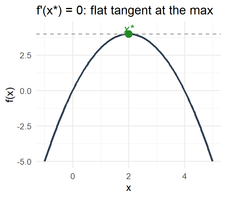
Then \(\nabla f(x^*)=0\).
An equivalent theorem holds for local minimum.
Critical point: Any point \(x^*\) that satisfies the first-order condition is called a critical point of \(f\) on \(D\).
What is the intuitive (geometric) proof of the above theorem?
What could be sufficient conditions? Hint: think about \(f''\).
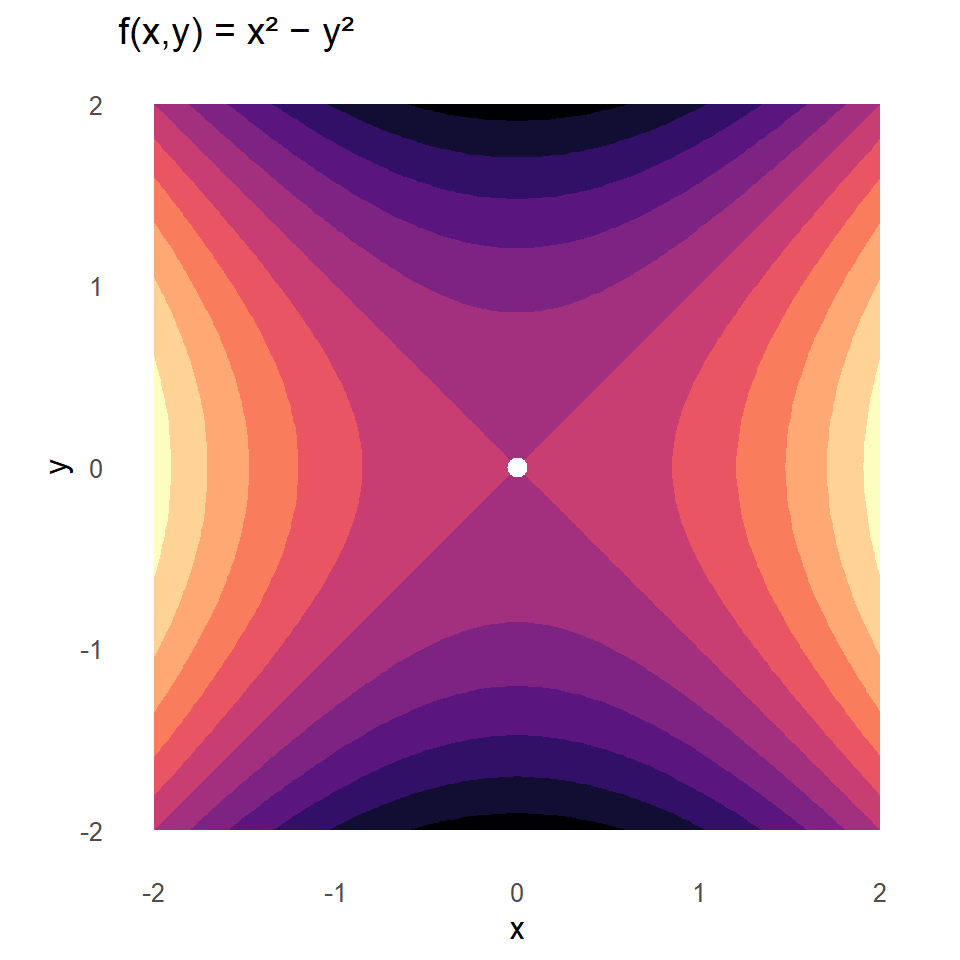
Avoiding the saddle point trap
Second-order conditions
First-order conditions do not distinguish between maxima, minima and saddle points. We need to examine the behavior of the second derivative \(\nabla^2f\) of \(f\) to conclude anything.
Theorem
- If \(f\) has a local maximum at \(x^*\in int(D)\), then \(\nabla^2f(x^*)\) is negative semidefinite.
- If \(f\) has a local minimum at \(x^*\in int(D)\), then \(\nabla^2f(x^*)\) is positive semidefinite.
- If \(\nabla f(x^*)=0\) and \(\nabla^2f(x^*)\) is negative definite, then \(x^*\) is a strict local maximum of \(f\) on \(D\).
- If \(\nabla f(x^*)=0\) and \(\nabla^2f(x^*)\) is positive definite, then \(x^*\) is a strict local minimum of \(f\) on \(D\).
In \(\mathbb{R}\), what is the equivalent of \(\nabla^2f(x^*)\) being negative definite?
Reminder
Positive (resp. negative) definiteness of a matrix
We say that a matrix \(M\in \mathbb{R}^{n\times n}\) is positive definite if \[\forall v\neq 0\in \mathbb{R}^{n}, v^\top M v >0.\]
We say that a matrix \(M\in \mathbb{R}^{n\times n}\) is negative definite if \[\forall v\neq 0\in \mathbb{R}^{n}, v^\top M v <0\]
We say it is positive semi-definite if \[\forall v\in \mathbb{R}^{n}, v^\top M v \geq 0\]
We say it is negative semi-definite if \[\forall v\in \mathbb{R}^{n}, v^\top M v \leq 0\]
Connecting the dots
Do you remember the formula for first-order Taylor expansion? For second order Taylor expansion?
General formula for differentiable function around \(x^*\):
\[f(x)\approx\sum_{|\alpha|\le k}\frac{D^\alpha f(x^*)}{\alpha!}\,(x - x^*)^\alpha\]
For second order-approximation:
\[f(x^* + \Delta x) - f(x^*)\;\approx\;\nabla f(x^*)^\top\,\Delta x + \frac{1}{2} \Delta x^\top\nabla^2 f(x^*)\,\Delta x\]
Connecting the dots
If the FOC are met: \[\nabla f(x^*) = 0\]
Thus:
\[f(x^* + \Delta x) - f(x^*)\;\approx\;\frac{1}{2} \Delta x^\top\nabla^2 f(x^*)\,\Delta x\]
And if \(\nabla^2 f(x^*)\) is positive definite (resp. negative definite), we have: \(\forall \Delta x, \Delta x^\top \nabla^2 f(x^*)\Delta x>0\) (resp. \(\forall \Delta x, \Delta x^\top \nabla^2 f(x^*)\Delta x<0\)).
And thus conclusions about the nature of \(x^*\) follow.
What is a sufficient condition for a local optimum to be a global optimum?
Concave and convex functions
Definition: Convexity and concavity in \(\mathbb{R}^n\)
A function \(f: \mathbb{R}^n \to \mathbb{R}\) is called convex if for all \(x,y \in \mathbb{R}^n\) and all \(\lambda \in [0,1]\), the following inequality holds:
\[f\bigl(\lambda x + (1-\lambda)y\bigr) \;\le\; \lambda\,f(x) \;+\; (1-\lambda)\,f(y).\]
It is called concave if
\[f\bigl(\lambda x + (1-\lambda)y\bigr) \;\ge\; \lambda\,f(x) \;+\; (1-\lambda)\,f(y).\]
(Unconstrained) local–global theorem
Theorem
Let \(f\) be a twice continuously differentiable real-valued concave function on \(D\). The following statements are equivalent, where \(x^*\) is an interior point of \(D\):
- \(\nabla f(x^*)=0\).
- \(f\) achieves a local maximum at \(x^*\).
- \(f\) achieves a global maximum at \(x^*\).
An analogue theorem with convex functions exists for minima.
What is the intuition behind this result?
Uniqueness of global optima
Theorem: Strict Concavity/Convexity and the Uniqueness of Global Optima
- If \(x^*\) maximizes the strictly concave function \(f\), then \(x^*\) is the unique global maximizer: \[f(x^*)>f(x)\quad \forall x\in D,\ x\neq x^*.\]
- If \(\tilde x\) minimizes the strictly convex function \(f\), then \(\tilde x\) is the unique global minimizer: \[f(\tilde x)<f(x)\quad \forall x\in D,\ x\neq \tilde x.\]
Constrained optimization with equality constraints
Motivation
In virtually all scenarios, you will face constraints in your choice, and these constraints will be binding (e.g. the now famous work / leisure tradeoff).
We will review how to solve these problems now.
Example: study–leisure tradeoff
Setup:
- Total time endowment: \(T\) hours.
- Choice variables: \(x_1 = \text{study hours},\ x_2 = \text{leisure hours}.\)
- Utility (Cobb–Douglas): \(U(x_1,x_2) = x_1^{\alpha}\,x_2^{1-\alpha},\quad 0<\alpha<1.\)
- Time constraint: \(x_1 + x_2 = T.\)
Constrained maximization: formalization for the substitution method
- \(f(x_1,x_2)\) is the objective function.
- \(x_1\) and \(x_2\) are choice variables.
- \(g(x_1,x_2)\) is the constraint, defining feasible values.
Substitution Method: If we can solve for \(x_2\) in terms of \(x_1\) (\(x_2=\tilde g(x_1)\)), and substitute:
\[\max_{x_1}f(x_1,\tilde g(x_1)).\]
Then, the problem becomes an unconstrained maximization problem.
The first-order condition becomes:
\[\frac{\partial f(x_1,\tilde g(x_1))}{\partial x_1}+\frac{\partial f(x_1,\tilde g(x_1))}{\partial x_2}\frac{d\tilde g(x_1)}{dx_1}=0.\]
Example: study–leisure tradeoff
Setup:
- Total time endowment: \(T\) hours.
- Choice variables: \(x_1 = \text{study hours},\ x_2 = \text{leisure hours}.\)
- Utility (Cobb–Douglas): \(U(x_1,x_2) = x_1^{\alpha}\,x_2^{1-\alpha},\quad 0<\alpha<1.\)
- Time constraint: \(x_1 + x_2 = T.\)
Who wants to try the substitution?
Substitution:
\[x_2 = T - x_1,\quad\max_{0\le x_1\le T} U\bigl(x_1,\,T - x_1\bigr)= \max_{x_1}\; x_1^{\alpha}(T - x_1)^{1-\alpha}.\]
First-Order Condition:
\[\frac{d}{dx_1}\bigl[x_1^{\alpha}(T - x_1)^{1-\alpha}\bigr]= \alpha\,x_1^{\alpha-1}(T - x_1)^{1-\alpha}\;-\;(1-\alpha)\,x_1^{\alpha}(T - x_1)^{-\alpha}= 0\]
\[\Leftrightarrow\;\alpha\,(T - x_1)\;=\;(1-\alpha)\,x_1\;\Leftrightarrow\;x_1 = \alpha T.\]
Interpretation: The optimal allocation splits time so that study receives fraction \(\alpha\) and leisure \((1-\alpha)\) of \(T\).
Lagrange’s method
Very often, constraint \(g\) sufficiently complicated so that you cannot find an explicit substitution. \(\Rightarrow\) Use Lagrange’s method!
Lagrange (1736-1813) started from the evidence: solving unconstrained problems is straightforward. Find partial derivatives, set them to zero, solve to get local optima.
…so maybe we should try to make the constrained problem an unconstrained one! The idea: Consider our original problem
\[\max_{x_1,x_2}f(x_1,x_2)\quad\text{subject to }g(x_1,x_2)=0.\]
Build the Lagrangian:
\[\mathcal{L}(x_1,x_2,\lambda)=f(x_1,x_2)-\lambda\,g(x_1,x_2).\]
Lagrange’s method: weak duality
And now optimize the Lagrangian. To understand in more depth the Lagrangian, you should check the literature on the duality principle. It basically consists in solving an easier problem (called the dual problem) rather than the original one (the primal problem).
With the Lagrangian, this is solving:
\[\max_{\lambda\geq0} \min_x \mathcal{L}(x,\lambda)\]
You will always have that:
\[\max_{\lambda\geq0} \min_x \mathcal{L}(x,\lambda) \leq \min_{x\text{ satisfies the constraints}} f(x)\]
\[\min_{\lambda\geq0} \max_x \mathcal{L}(x,\lambda) \geq \max_{x\text{ satisfies the constraints}} f(x)\]
A result known as weak duality.
Lagrange’s method: strong duality
We say that strong duality is satisfied if
\[\max_{\lambda\geq0} \min_x \mathcal{L}(x,\lambda) = \min_{x\text{ satisfies the constraints}} f(x)\]
\[\min_{\lambda\geq0} \max_x \mathcal{L}(x,\lambda) = \max_{x\text{ satisfies the constraints}} f(x)\]
In this case, we may only solve the dual problem.
Lagrange’s method: strong duality
In practice, during the master’s, you will mostly (if not only) meet cases where strong duality holds. A sufficient condition for strong duality is known as:
Theorem: Slater’s condition
Assume you have a convex (concave) objective function \(f(x); \mathbb{R}^n\mapsto\mathbb{R}\) defined over a convex domain \(\mathcal{D}\), and constraints defined by functions \(g_i(x)\) and \(h_j(x)\) of the form \(g_i(x)\leq 0, h_i(x)=0\). If:
- \(\forall i, g_i\) is convex;
- \(\forall j, h_j\) is affine;
- there exists at least 1 point \(x\) strictly satisfying all the constraints (i.e. \(\forall i g_i\leq 0\) and \(g_i<0\) for non-affine \(g_i\), \(\forall j\, h_j(x)=0\));
Then strong duality holds (i.e. solving the dual is the same as the primal problem).
You may read the book by Boyd & Vandenberghe (2004) if you want to go further (but it is not needed). It is freely available online.
Lagrange’s method: solving the problem
Under affine equality constraints, solving the Lagrangian problem is thus sufficient!
Critical Points of \(\mathcal{L}\):
\[\frac{\partial\mathcal{L}}{\partial x_1}=\frac{\partial f(x_1,x_2)}{\partial x_1}-\lambda\,\frac{\partial g(x_1,x_2)}{\partial x_1}=0,\]
\[\frac{\partial\mathcal{L}}{\partial x_2}=\frac{\partial f(x_1,x_2)}{\partial x_2}-\lambda\,\frac{\partial g(x_1,x_2)}{\partial x_2}=0,\]
\[\frac{\partial\mathcal{L}}{\partial \lambda}=g(x_1,x_2)=0.\]
Outcome: If we find \(x_1^*,x_2^*,\lambda^*\) satisfying these, we locate a critical point. Note that the third condition is the constraint.
Back to the study–leisure tradeoff example
Preferences & Constraint
\[\max_{x_1,x_2}\; U(x_1,x_2) = x_1^{\alpha} \, x_2^{1-\alpha},\quad 0<\alpha<1,\quad x_1 + x_2 = T\]
Lagrangian
\[\mathcal{L}(x_1,x_2,\lambda)= x_1^{\alpha} x_2^{1-\alpha}- \lambda\,(x_1 + x_2 - T).\]
First-Order Conditions
\[\frac{\partial \mathcal{L}}{\partial x_1}= \alpha x_1^{\alpha-1} x_2^{1-\alpha} - \lambda = 0,\quad\frac{\partial \mathcal{L}}{\partial x_2}= (1-\alpha) x_1^{\alpha} x_2^{-\alpha} - \lambda = 0,\quad\frac{\partial \mathcal{L}}{\partial \lambda}= T - x_1 - x_2 = 0.\]
Solving the FOCs: divide the 2 first FOCs
\[\frac{\alpha x_1^{\alpha-1} x_2^{1-\alpha}}{(1-\alpha) x_1^{\alpha} x_2^{-\alpha}}= 1\;\Longrightarrow\;\frac{\alpha}{1-\alpha} \frac{x_2}{x_1} = 1\;\Longrightarrow\;x_2 = \frac{1-\alpha}{\alpha} \, x_1.\]
Time-Budget Constraint
\[x_1 + x_2 = T\;\Longrightarrow\;x_1^* = \alpha \, T,\quad x_2^* = (1-\alpha) \, T.\]
Value of \(\lambda\).
\[\lambda^* = \alpha (\alpha T)^{\alpha-1} ((1-\alpha)T)^{1-\alpha}= \alpha^{\alpha} (1-\alpha)^{1-\alpha}.\]
Numerical Illustration
\[\alpha = 0.5,\; T = 16\ \text{hours}\quad\Longrightarrow\quad x_1^* = 8,\quad x_2^* = 8,\quad\lambda = 0.5\]
The student optimally allocates 8 hours to study (\(x_1\)) and 8 hours to leisure (\(x_2\)).
Interpretation of the multiplier, \(\lambda\)
The Lagrange multiplier has a profound economic interpretation:
- It measures the rate at which the maximum value of \(f\) would increase if the constraint \(g\) were relaxed slightly.
- If \(\lambda=0\), the constraint is non-binding (i.e., not affecting the outcome), and the problem is an unconstrained maximization.
- In economic terms, \(\lambda\) is called the “shadow price” or “marginal value” of relaxing the constraint.
Interpretation of the multiplier: example
In the previous example we have:
\[U(x_1^*,x_2^*) = 0.5^{0.5} \cdot 0.5^{0.5} \times 16 = \sqrt{0.25} \times 16 = 8\]
If \(T\) increased by one unit, we would have:
\[U(x_1^*,x_2^*) = 0.5^{0.5} \cdot 0.5^{0.5} \times 17 = \sqrt{0.25} \times 17 = 8.5\]
This represents an increase of 0.5 in utility.
…exactly the value of \(\lambda\)!
The envelope theorem: unconstrained case
Theorem: Envelope theorem (unconstrained optimization)
If \(x^*(\theta)\) is an interior maximizer and both \(f\) and \(x^*(\cdot)\) are \(C^1\), then \[V'(\theta)=\frac{\partial f}{\partial \theta}\bigl(x^*(\theta),\theta\bigr).\]
Proof (chain rule): \[V'(\theta)=\underbrace{\nabla_x f(x^*(\theta),\theta)^\top}_{=\,0\ \text{by the FOC}}\,\frac{dx^*}{d\theta}+\frac{\partial f}{\partial\theta}(x^*(\theta),\theta).\]
At an optimum the indirect effect (re-optimizing \(x\)) is second-order. You only need the direct effect of \(\theta\) on the objective.
The envelope theorem: constrained case
\[V(\theta)=\max_x f(x,\theta)\quad\text{s.t. } g_j(x,\theta)=0,\ j=1,\dots,m.\]
Theorem: Envelope theorem (Lagrangian form)
Under the assumptions of Lagrange’s theorem, with \((x^*(\theta),\lambda^*(\theta))\) \(C^1\): \[V'(\theta)=\frac{\partial \mathcal{L}}{\partial\theta}\bigl(x^*(\theta),\lambda^*(\theta)\bigr) =\frac{\partial f}{\partial\theta}(x^*,\theta)-\sum_{j=1}^m\lambda_j^*\,\frac{\partial g_j}{\partial\theta}(x^*,\theta).\]
Differentiate the Lagrangian, not the objective: the constraint moves too, and \(\lambda^*\) prices that movement.
Back to study–leisure. Here \(\theta=T\) and \(g(x,T)=x_1+x_2-T\), so \(\partial f/\partial T=0\) and \(\partial g/\partial T=-1\): \[V'(T)=0-\lambda^*(-1)=\lambda^*=\alpha^\alpha(1-\alpha)^{1-\alpha}=0.5 .\]
So the “+0.5 utility per extra hour” from two slides ago was not a numerical accident: the shadow-price interpretation of \(\lambda\) comes from the envelope theorem!
Lagrange’s theorem
Theorem: Lagrange’s Theorem
Let \(f(x)\) and \(g_j(x),\,j=1,\dots,m\), be \(C^1\) real-valued functions over some domain \(D\subset\mathbb{R}^n\). Let \(x^*\) be an interior point of \(D\), and suppose that \(x^*\) is an optimum of \(f\) subject to \(g_j(x^*)=0,\ j=1,\dots,m\).
If the gradient vectors \(\nabla g_j(x^*)\) are linearly independent, then there exist unique \(\lambda_j^*,\,j=1,\dots,m\), such that
\[\frac{\partial \mathcal{L}(x^*,\lambda^*)}{\partial x_i}=\frac{\partial f(x^*)}{\partial x_i}-\sum_{j=1}^m\lambda_j^*\,\frac{\partial g_j(x^*)}{\partial x_i}=0,\quad i=1,\dots,n.\]
In the theorem, I use another condition than the Slater’s condition. Which one?
Are we guaranteed that the critical point be a local maximum / minimum?
The scenarios with a derivative equal 0
- Minimum;
- Maximum;
- Saddle point.
Second-order conditions: local optimality
Let \(f\) be defined on an open set \(D\subset\mathbb{R}^n\), differentiable in each variable. Let \(H\) denote the Hessian matrix of \(f\) at \(x^*\). Do you remind the definition of the Hessian matrix? And why it might be interesting?
\[H_f(x^*)=\Bigl[\frac{\partial^2 f}{\partial x_i\,\partial x_j}(x^*)\Bigr]_{i,j=1}^n=\begin{pmatrix}\displaystyle\frac{\partial^2 f}{\partial x_1^2}(x^*)& \cdots &\displaystyle\frac{\partial^2 f}{\partial x_1\,\partial x_n}(x^*)\\\vdots & \ddots & \vdots\\\displaystyle\frac{\partial^2 f}{\partial x_n\,\partial x_1}(x^*)& \cdots &\displaystyle\frac{\partial^2 f}{\partial x_n^2}(x^*)\end{pmatrix}.\]
Do you think we should use this Hessian to conclude about local optimality?
Yes, you can… but you should not! As there are constraints, some of the \(\Delta x\) might be unfeasible, and we need to acknowledge this. We only need that the Hessian be definite in the “constraint space”, not that the Hessian be definite on the full domain of \(f\). One strategy we will not discuss would thus be to project the Hessian matrix onto the tangent space of the constraints.
Local optimality: the bordered Hessian
The bordered Hessian matrix is the Hessian matrix of the Lagrangian associated with the optimization problem. For an objective function \(f: \mathbb{R}^n\mapsto\mathbb{R}\) and constraints \(g: \mathbb{R}^n\mapsto\mathbb{R}^m\), it is a matrix of the form:
\[H_\mathcal{L}(x,\lambda)=\begin{pmatrix}\nabla^2_{\lambda\lambda}\mathcal{L}(x,\lambda) & (\nabla^2_{\lambda x}\mathcal{L}(x,\lambda))^T \\\nabla^2_{x \lambda}\mathcal{L}(x,\lambda) & \nabla^2_{xx}L(x,\lambda)\end{pmatrix},\]
Recall the Lagrangian is: \(\mathcal{L}(x,\lambda)=f(x)-\lambda\,g(x).\)
From this, can you tell what will be in each of the corners of the matrix?
Local optimality: the bordered Hessian
Recall the Lagrangian is: \(\mathcal{L}(x,\lambda)=f(x)-\lambda\,g(x).\)
Thus, you have:
\[\nabla^2_{\lambda\lambda}\mathcal{L}(x,\lambda) = 0_{m\times m}\]
\[\nabla^2_{\lambda x}\mathcal{L}(x,\lambda) = \nabla^2_{x \lambda}\mathcal{L}(x,\lambda) = \nabla g(x)\]
Hence:
\[H_\mathcal{L}(x,\lambda)=\begin{pmatrix}0_{m\times m} & (\nabla g(x) )^T \\\nabla g(x) & \nabla^2_{xx}\mathcal{L}(x,\lambda)\end{pmatrix}\]
A notion we will need: principal minors
Definition
Let \(A\) be an \(n\times n\) matrix. The \(k\)th order principal submatrix of \(A\), obtained by deleting the last \(n-k\) rows and the last \(n-k\) columns from \(A\), is called the \(k\)th order leading principal submatrix of \(A\). Its determinant is called the \(k\)th order leading principal minor of \(A\). We denote the \(k\)th order leading principal submatrix by \(A_k\) and the corresponding leading principal minor by \(|A_k|\).
Concluding from the bordered Hessian
Theorem
Let \(f:\mathbb{R}^n\to\mathbb{R}\) be the objective function to be maximized and \(g:\mathbb{R}^n\to\mathbb{R}^m\) represent constraints. Form the Lagrangian \(\mathcal{L}(x,\lambda)= f(x)\;-\;\lambda^T\,g(x),\) and let \((x^*,\lambda^*)\) be a critical point. Denote the bordered Hessian \(H\) and assume constraints are not degenerate (i.e. \(\nabla g(x^*)\) has full rank \(m\)). To determine the definiteness of \(f\) on the constraint space formed by \(g(x)\), inspect the signs of the last \(n-m\) leading principal minors of \(H\), beginning with \(\det H\):
- If \(\det H\) has the same sign as \((-1)^n\) and the last \(n-m\) minors alternate in sign, then \(f\) has a strict local maximum at \(x^*\) on \(\{x:g(x)=0\}\).
- If \(\det H\) and the last \(n-m\) minors all have the same sign as \((-1)^m\), then \(f\) has a strict local minimum at \(x^*\) on \(\{x:g(x)=0\}\).
- If neither pattern holds, then \(f\) is indefinite on \(\{x:g(x)=0\}\), and \(x^*\) is neither a local maximum nor a local minimum on the constraint set.
Checking global optimality
- Local optimality doesn’t always imply global optimality.
- Convex (concave) functions over convex domains: local minima (maxima) are global.
- Without special properties, determining global optimality can be challenging.
Takeaway: While second-order conditions provide clarity about local behavior, global optimality often requires deeper examination or additional assumptions.
Example 19.8 in Simon & Blume
Consider the problem of maximizing \(x^2y^2z^2\) subject to the constraint \(x^2+y^2+z^2=3\). What is the Lagrangian?
\[\mathcal{L}=x^2y^2z^2-\mu(x^2+y^2+z^2-3)\]
It yields the FOCs:
\[\frac{\partial L}{\partial x} = 2xy^2z^2-2\mu x = 0\]
\[\frac{\partial L}{\partial y} = 2x^2yz^2-2\mu y = 0\]
\[\frac{\partial L}{\partial z} = 2x^2y^2z-2\mu z = 0\]
\[-\frac{\partial L}{\partial \mu} = x^2+y^2+z^2-3 = 0\]
Solving the FOCs step by step
First-order conditions:
\[\frac{\partial L}{\partial x}=2xy^2z^2-2\mu x=0,\quad\frac{\partial L}{\partial y}=2x^2yz^2-2\mu y=0,\quad\frac{\partial L}{\partial z}=2x^2y^2z-2\mu z=0,\]
\[\frac{\partial L}{\partial \mu}=-(x^2+y^2+z^2-3)=0.\]
Can you find a trick to solve the problem?
The objective \(x^2y^2z^2\ge 0\) and note that \((1,1,1)\) is a feasible point with \(f(1,1,1)=1>0\). Therefore, no maximizer can have any of \(x,y,z\) equal to \(0\). Since \(x,y,z\neq 0\), we may divide the FOCs.
Solving the FOC
\[y^2z^2=\mu,\qquad x^2z^2=\mu,\qquad x^2y^2=\mu.\]
Equating these gives
\[y^2z^2=x^2z^2 \;\Rightarrow\; x^2=y^2,\qquad x^2z^2=x^2y^2 \;\Rightarrow\; y^2=z^2\;\Rightarrow\; x^2=y^2=z^2=:t.\]
Using the constraint \(x^2+y^2+z^2=3\),
\[3t=3 \;\Rightarrow\; t=1 \;\Rightarrow\; x^2=y^2=z^2=1,\quad\text{and}\quad \mu=y^2z^2=t^2=1.\]
Thus the only point satisfying the FOC is \((x,y,z) = (1,1,1)\).
Ensuring local maximum
With solution \(x^2=y^2=z^2=\mu=1\). The bordered Hessian for this problem is
\[\begin{pmatrix}0 & 2x & 2y & 2z\\2x & 2y^2z^2-2\mu & 4xyz^2 & 4xy^2z\\2y & 4xyz^2 & 2x^2z^2-2\mu & 4x^2yz\\2z & 4xy^2z & 4x^2yz & 2x^2y^2-2\mu\end{pmatrix}.\]
Ensuring local maximum
At \(x=y=z=\mu=1\), the bordered Hessian becomes:
\[\begin{pmatrix}0 & 2 & 2 & 2 \\2 & 0 & 4 & 4 \\2 & 4 & 0 & 4 \\2 & 4 & 4 & 0\end{pmatrix}\]
Since \(n=3\) and \(m=1\), we have to check the signs of two leading principal minors: the \(3\times 3\) submatrix \(H_3\) in the top-left corner and the complete \(4\times 4\) matrix. One computes that \(\det H_3=32\) and \(\det H_4=-192\). Since these determinants alternate in sign and since the sign of \(\det H_4\) is the sign of \((-1)^3=-1\), the candidate \(x=y=z=1\) is a locally unique solution to our problem.
Constrained optimization with inequality constraints
The simplest complexified problem – non-negativity constraints
Most of the time, you will face neither equality constraints nor unconstrained problems, but rather have constraints in the form of inequality. We start with simple non-negativity constraints.
Let’s define the problem:
\[\max_x f(x)\quad\text{subject to }x\ge0.\]
Assuming \(f\) is strictly concave, derive the conditions characterizing the solution \(x^*\).
Possible cases
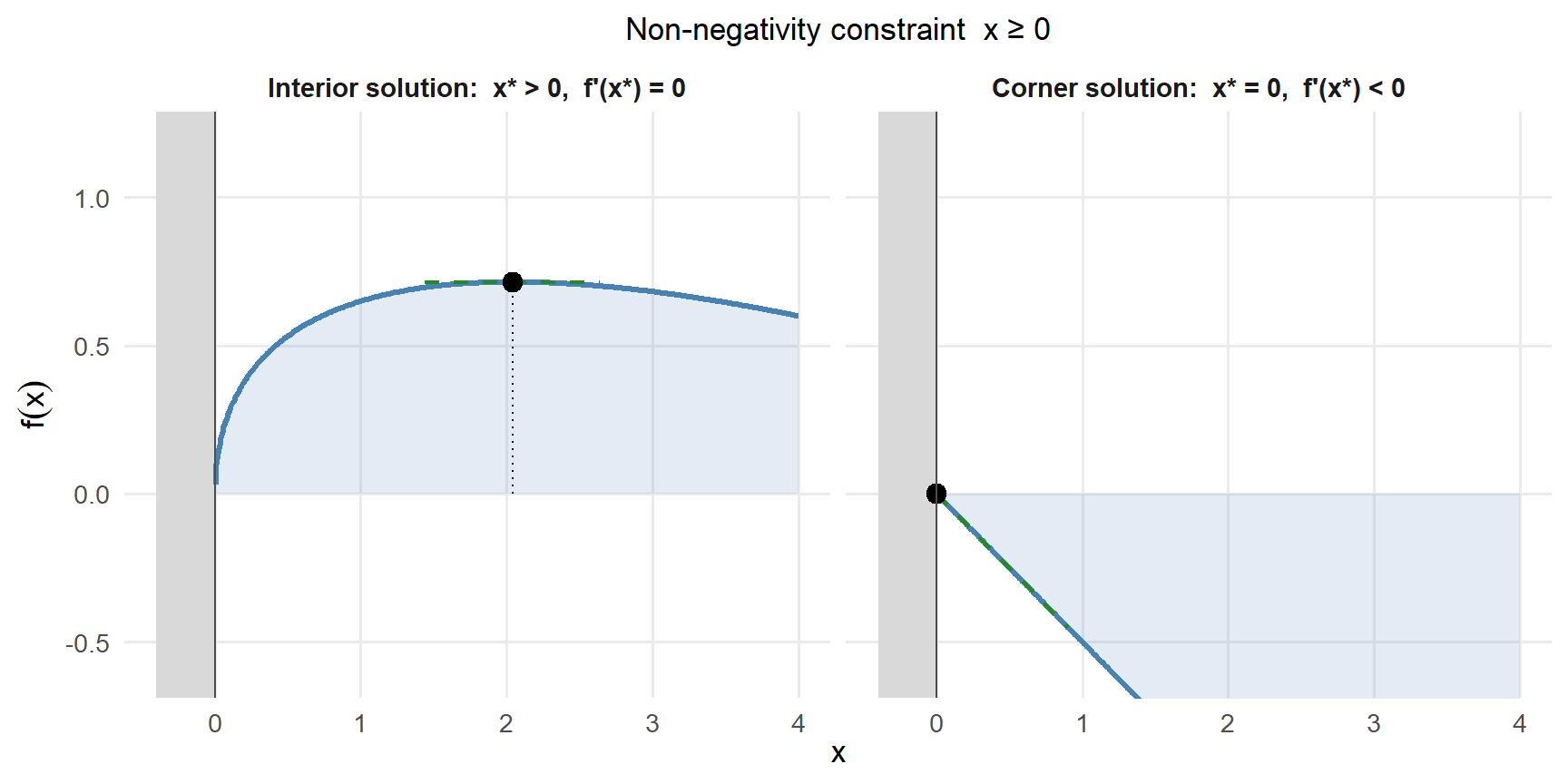
For optimality, what are the joint possible cases regarding (i) the value of critical points \(x^*\) and (ii) \(f'(x^*)\)?
From cases to conditions
The three possible cases are:
- \(x^*=0\) and \(f'(x)<0\).
- \(x^*=0\) and \(f'(x)=0\).
- \(x^*>0\) and \(f'(x)=0\).
What is the common theme?
In all three cases, \(x^*\,f'(x)=0 \Rightarrow\) this should be part of the condition for a solution.
From cases to conditions
However, that is not enough. Consider \(\tilde x=0\) and \(f'(x)>0\). Clearly not a maximum, yet it respects \(x^*f'(x)=0\).
The solution is characterized by:
\[\begin{cases}\text{Condition 1. }f'(x)\le0,\\\text{Condition 2. }x^*f'(x)=0,\\\text{Condition 3. }x^*\ge0.\end{cases}\]
The simple problem’s key condition
Recall:
\[\begin{cases}f'(x)\le0,\\x^*f'(x)=0,\\x^*\ge0.\end{cases}\]
- If \(x^*=0\), the constraint binds and \(f'(x^*)\le0\).
- If \(x^*>0\), it must stationary: \(f'(x^*)=0\).
We set the stage for the more general problem… and will again use the Lagrangian.
Setting the stage: the general problem
\[\max_x f(x)\quad\text{subject to }g_i(x)\le0,\ i=1,\dots,m, \qquad h_j(x)=0,\ j=1,\dots,l.\]
Lagrangian:
\[\mathcal{L}(x,\mu)=f(x)-\sum_{i=1}^m\lambda_i\,g_i(x)-\sum_{i=1}^l\mu_i\,h_j(x).\]
Here, \(\lambda,\mu\) are Lagrange multipliers. When constraints bind (\(g_i(x)=0\)), they adjust the Lagrangian to stay feasible. In the next few slides: conditions under which the problem can be solved.
Condition 1: primal feasibility
The first condition we need… is that the constraints are satisfied:
\[g_i(x)\le0,\quad i=1,\dots,m\qquad h_j(x)=0,\ j=1,\dots,l.\]
This is called primal feasibility because the points satisfying the condition are in the constraint set of the primal problem.
Condition 2: dual feasibility
The second condition we need is that the dual is solved, and thus that Lagrange multipliers \(\lambda_i\) satisfy:
\[\lambda_i\ge0,\quad i=1,\dots,m.\]
This is dual feasibility.
Reason: A negative \(\lambda_i\) would counteract \(g_i(x)\le0\). To preserve direction, require \(\lambda_i\ge0\).
Condition 3: complementary slackness
The third condition is just that the problem is at optimum: either the constraint binds, or the constraint does not bind and we have a derivative equal 0 at an interior point:
\[\lambda_i\,g_i(x)=0,\quad i=1,\dots,m.\qquad \mu_j\,h_j(x)=0,\quad i=1,\dots,l.\]
If \(\mu_i\neq0\), constraint binding; else not influencing.
Condition 4: stationarity
The last condition is just that the derivative of the Lagrangian wrt to the choice variables \(x\) be 0.
\[\nabla f(x)-\sum_{i=1}^m\lambda_i\nabla g_i(x)-\sum_{i=1}^l\mu_i\nabla h_i(x)=0.\]
Note: slack constraints do not matter for stationarity since their associated Lagrange multipliers are 0… so sometimes you might be clever in finding the intuition why some constraints should bind / not bind to make easier the computations.
KKT necessary conditions
Theorem: KKT Necessary Conditions
Let \(f,g_i,h_j\) be \(C^1\) functions. Suppose at a local maximizer \(x^*\), a constraint qualification holds (e.g. next slide). Then there exist multipliers \((\lambda^*,\mu^*)\) with \(\lambda^*\ge 0\) such that the KKT conditions hold at \((x^*,\lambda^*,\mu^*)\).
Takeaway: With a CQ, every local maximum must satisfy KKT; without a CQ, KKT may fail even at optima. ( i.e. strong duality does not hold)
“Karush–Kuhn–Tucker (KKT) conditions” and “Karush–Kuhn–Tucker (KKT) Lagrangian” are tribute to the researchers who studied it.
Constraint qualifications (CQs)
All the following are valid constraint qualifications.
- LICQ: Gradients of active constraints at \(x^*\) are linearly independent.
- MFCQ: Equalities are independent and there exists a direction strictly decreasing all active inequalities.
- Slater’s condition.
When are KKT sufficient?
Theorem: KKT Necessary & Sufficient
Consider the maximization problem with \(f\) concave, each \(g_i\) convex, and each \(h_j\) affine. If Slater’s condition holds, then a point \(x^*\) is a global maximizer if and only if there exist multipliers \((\lambda^*,\mu^*)\) with \(\lambda^*\ge 0\) such that the KKT conditions hold at \((x^*,\lambda^*,\mu^*)\).
Takeaway: In convex optimization (concave maximization), first-order KKT fully characterizes global optimality.
Second-order sufficient conditions
Theorem: Second-Order Sufficient Condition
Let \(x^*\) be a feasible point for the maximization problem, and suppose there exists \(\lambda^*\) such that the KKT conditions hold at \((x^*,\lambda^*)\). Let
\[C(x^*,\lambda^*) = \left\{ w \in \mathbb{R}^n \; : \;\nabla h_j(x^*)^\top w = 0, \;\nabla g_i(x^*)^\top w = 0 \ \forall i \text{ s.t. }\lambda_i^* > 0\right\}\]
be the critical cone. If
\[w^\top \nabla^2_{xx} \mathcal{L}(x^*,\lambda^*) \, w < 0\quad \text{for all } w \in C(x^*,\lambda^*), \; w \neq 0,\]
then \(x^*\) is a strict local maximizer.
Note that the bordered Hessian test also works.
When constraints don’t bind
- If \(g_i(x)\le0\) doesn’t affect optimum, treat as if it doesn’t exist.
- Corresponding \(\mu_i=0\) “switches off” the constraint.
Implication: Unconstrained world despite listed constraints.
When constraints bind
- A binding \(g_i(x)=0\) acts like an equality constraint.
- \(\mu_i\neq0\) is the “penalty” for marginal violation.
Implication: Optimization respects the constraint, adjusting the objective.
Example: problem statement
Goal. Solve a constrained maximization with KKT.
Primal problem:
\[\max_{x_1,x_2>0} \; f(x_1,x_2) = \ln x_1 + \ln x_2\]
subject to
\[\underbrace{2x_1 + x_2 \le 10}_{\text{budget}},\qquad\underbrace{x_1 \ge 3}_{\text{minimum requirement}},\qquad\underbrace{x_2 \ge 0}_{\text{nonnegativity}}.\]
Economic reading: Cobb–Douglas utility; prices \((p_1,p_2)=(2,1)\), income \(I=10\), and a policy minimum \(x_1\ge 3\) (e.g. you must eat a decent amount of food).
Why KKT theorem applies (sufficiency)
- Objective \(\ln x_1 + \ln x_2\) is strictly concave on \(x_i>0\).
- Feasible set is an intersection of half-spaces \(\Rightarrow\) convex.
- The problem respects Slater’s condition: constraints are convex and there exists a strictly feasible point with \(g_i(x)<0\) for all \(i\) (e.g. \((x_1,x_2)=(3.1,1)\) satisfies \(2x_1+x_2<10\), \(x_1>3\), \(x_2>0\)).
- Concavity + Slater \(\Rightarrow\) KKT conditions are necessary and sufficient, and the solution is unique.
Put constraints in KKT form
Write all constraints as \(g_i(x)\le 0\):
\[g_b(x)= 2x_1 + x_2 - 10 \le 0 \quad\text{(budget)}\]
\[g_m(x)= 3 - x_1 \le 0 \quad\text{(minimum)}\]
\[g_n(x)= -x_2 \le 0 \quad\text{(nonnegativity)}\]
Multipliers \(\lambda,\mu,\nu\ge 0\) will be associated with \(g_b,g_m,g_n\) respectively.
Lagrangian and KKT system
Lagrangian:
\[\mathcal{L}(x_1,x_2,\lambda,\mu,\nu)= \ln x_1 + \ln x_2 - \lambda\,(2x_1+x_2-10) - \mu\,(3-x_1) - \nu\,(-x_2).\]
Stationarity:
\[\partial_{x_1}\mathcal{L}= \frac{1}{x_1} - 2\lambda + \mu = 0,\qquad\partial_{x_2}\mathcal{L}= \frac{1}{x_2} - \lambda + \nu = 0.\]
Primal feasibility: \(2x_1+x_2\le 10,\; x_1\ge 3,\; x_2\ge 0\).
Dual feasibility: \(\lambda,\mu,\nu\ge 0\).
Complementary slackness:
\[\lambda\,[2x_1+x_2-10]=0, \qquad \mu\,[3-x_1]=0, \qquad \nu\,[-x_2]=0.\]
Step 1: check whether some constraints should not bind
Non-negativity does not bind: If non-negativity binds, we have infinite disutility, so we should have strict inequality. Hence, we should have \(\nu=0\).
Budget binds: the objective is strictly increasing so the more the better. The constraint must bind.
Expenditure minimum may bind depending on relative prices: let’s solve the unconstrained problem to find out. Without constraints, we should have equal expenditure for each good.
With prices \((2,1)\), equal expenditure shares imply \(2x_1 = x_2\). If the budget binds:
\[2x_1 + x_2 = 10 \;\Rightarrow\; 2x_1 + 2x_1 = 10 \Rightarrow x_1 = 2.5,\; x_2=5.\]
Observation: This point satisfies all constraints except \(x_1\ge 3\).
Because \(x_1=2.5\) violates the minimum, we expect \(x_1=3\) to bind at the true optimum.
Step 2: identify the active set
The active (binding) constraints are:
\[\boxed{x_1=3}, \qquad \boxed{2x_1 + x_2 = 10}, \qquad (x_2>0 \Rightarrow \text{nonnegativity is slack}).\]
Complementary slackness suggests \(\mu>0\), \(\lambda>0\), and \(\nu=0\).
Step 3: solve for multipliers
Plug \(x_1=3\), \(x_2=4\), \(\nu=0\) into stationarity:
\[\frac{1}{4} - \lambda + 0 = 0 \quad\Rightarrow\quad \boxed{\lambda=\tfrac{1}{4}},\]
\[\frac{1}{3} - 2\lambda + \mu = 0 \quad\Rightarrow\quad \boxed{\mu = 2\lambda - \tfrac{1}{3} = \tfrac{1}{6}}\;\;(\ge 0).\]
All KKT conditions are satisfied.
Solution and verification
Primal solution
\[\boxed{\;x_1^{\star}=3,\quad x_2^{\star}=4\;}.\]
Multipliers (shadow values)
\[\boxed{\;\lambda=\tfrac{1}{4},\quad \mu=\tfrac{1}{6},\quad \nu=0\;}.\]
Checks: Budget: \(2(3)+4=10\) (binds). Minimum: \(x_1=3\) (binds). Nonnegativity: \(x_2=4>0\) (slack). Stationarity holds by construction.
Economic interpretation
- \(\lambda\) (budget): increasing the RHS of \(2x_1+x_2\le 10\) by 1 raises maximal utility by \(\,\tfrac{\partial V}{\partial 10}=\lambda=\tfrac{1}{4}\).
- \(\mu\) (minimum): tightening the requirement to \(x_1\ge 3+\varepsilon\) reduces maximal utility at rate \(\mu\,\varepsilon = \tfrac{1}{6}\,\varepsilon\).
- \(\nu=0\) because \(x_2>0\), so the nonnegativity constraint is slack and carries no shadow value at the optimum.
Brute force
Lagrangian:
\[\mathcal L = \ln x_1 + \ln x_2 + \lambda(10 - 2x_1 - x_2)+ \mu_1(x_1 - 3)+ \mu_2 x_2\]
with \(\lambda, \mu_1, \mu_2 \ge 0\).
Stationarity:
\[\frac{\partial \mathcal L}{\partial x_1}:\quad \frac{1}{x_1} - 2\lambda + \mu_1 = 0\]
\[\frac{\partial \mathcal L}{\partial x_2}:\quad \frac{1}{x_2} - \lambda + \mu_2 = 0\]
Complementary slackness:
\[\lambda(10 - 2x_1 - x_2) = 0,\quad\mu_1(x_1 - 3) = 0,\quad\mu_2 x_2 = 0\]
Express \(x_1, x_2\) in terms of multipliers
From stationarity:
\[x_1 = \frac{1}{2\lambda - \mu_1}, \quad x_2 = \frac{1}{\lambda - \mu_2}\]
Primal feasibility requires \(2\lambda > \mu_1\) and \(\lambda > \mu_2\) (otherwise, \(x_i\) could be negative).
\(x_2>0\) is straightforward, complementary slackness thus gives:
\[\mu_2 = 0 \quad \Rightarrow \quad x_2 = \frac{1}{\lambda}.\]
And so budget must bind, otherwise \(x_2\) would take infinite value.
Case analysis
Case 1: \(x_1 > 3 \Rightarrow \mu_1 = 0\)
Then \(x_1 = \frac{1}{2\lambda}\). Budget binding:
\[2\left( \frac{1}{2\lambda} \right) + \frac{1}{\lambda} = \frac{2}{\lambda} = 10\quad\Rightarrow\quad \lambda = \frac{1}{5}\]
This gives \(x_1 = 2.5 < 3\) — contradiction.
Case 2: \(x_1 = 3 \Rightarrow\) constraint binds (\(\mu_1 > 0\))
Budget binding: \(2(3) + x_2 = 10 \quad\Rightarrow\quad x_2 = 4\)
From \(x_2 = \frac{1}{\lambda}\): \(\lambda = \frac{1}{4}\)
From stationarity in \(x_1\):
\[\frac{1}{3} - 2\left(\frac{1}{4}\right) + \mu_1 = 0\quad\Rightarrow\quad \mu_1 = \frac{1}{6}\]
Envelope theorem with inequality constraints
\[V(\theta)=\max_x f(x,\theta)\ \ \text{s.t.}\ \ g_i(x,\theta)\le 0,\ \ h_j(x,\theta)=0 .\]
We now have constraints that may or may not bind. Does that break the chain-rule argument?
Theorem: Envelope theorem (KKT form)
Let \((x^*(\theta),\lambda^*(\theta),\mu^*(\theta))\) satisfy the KKT conditions. Suppose LICQ holds, the second-order sufficient condition holds, and strict complementarity holds (\(\lambda_i^*>0\) for every active \(g_i\)). Then \(x^*,\lambda^*,\mu^*\) are \(C^1\) near \(\theta\), and
\[V'(\theta)=\frac{\partial\mathcal{L}}{\partial\theta} \bigl(x^*(\theta),\lambda^*(\theta),\mu^*(\theta)\bigr) =\frac{\partial f}{\partial\theta} -\sum_{i=1}^m\lambda_i^*\frac{\partial g_i}{\partial\theta} -\sum_{j=1}^l\mu_j^*\frac{\partial h_j}{\partial\theta}.\]
Same formula as before. Slack constraints contribute nothing: \(\lambda_i^*=0\) kills their term. Only the active set prices into \(V'\).
What the multipliers now mean
Write the constraints with an explicit right-hand side, \(g_i(x)\le c_i\). Then
\[\frac{\partial V}{\partial c_i}=\lambda_i^*\ \ge 0 .\]
Scarcity pricing
- Binding constraint \(\Rightarrow \lambda_i^*>0\): the resource is scarce, and \(\lambda_i^*\) is what one more unit is worth to you.
- Slack constraint \(\Rightarrow \lambda_i^*=0\): you would pay nothing for more of it. It is not scarce for you, at this optimum.
This is the whole logic of a shadow price: complementary slackness says a good is either scarce or free. You will meet the same statement again as the condition for a market to clear, as the price of a rationed good, and as the cost of a policy constraint.
When multiplier is not identified
A simple example: baking. Assume every cake needs exactly one egg and one cup of flour. You have \(E\) eggs and \(F\) cups of flour, so you can bake
\[V(E,F)=\min\{E,\,F\}\ \text{ cakes.}\]
You currently hold \(E=F=10\). Both constraints bind: no eggs left over, no flour left over.
I give you one more egg. How many extra cakes?
Zero. You have run out of flour.
I take one egg away. How many cakes do you lose?
One. Now the eggs are what stops you.
The answer depends on the direction
An egg is worth \(0\) if you are gaining one, and \(1\) if you are losing one. There is no single number “the value of an egg” — so there is no single multiplier \(\lambda_{\text{egg}}\).
Ties, kinks, and multipliers
Fix \(F=10\) and vary the eggs. The value function is \(V(E)=\min\{E,10\}\):
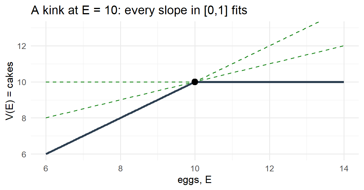
The multiplier is trying to be the slope of \(V\). To the left the slope is \(1\); to the right it is \(0\). At the kink, every dashed line in between touches the graph without crossing it… and every one of those slopes solves the KKT system.
The diagnostic, in one line
Tied constraints \(\Rightarrow\) many multipliers \(\Rightarrow\) kink in \(V\). The envelope formula still holds on each side separately, just with different multipliers left and right.
Here: only MFCQ holds, not LICQ.
Questions?
What will be useful for what?
Mathematical logic: cornerstone in econ. Important for micro I (likely to start with abstract definitions of what are the properties of “preferences”).
From the calculus session
- Continuity: virtually always assumed, never proved \(\rightarrow\) know intuitively what it is, and that theorems very often rely on it.
- Derivatives, gradients, jacobians and hessians: ubiquitous in micro (including micro I, although likely rather for part 2 of the semester).
- Sequences: they appear everywhere in econometrics 2 (but unsure you will have to prove anything about it), and for central limit theorem in metrics 1.
- Taylor’s theorem: very useful trick, underlies shortcuts you will likely take in macroeconomics.
- Log-linearization: ubiquitous in macroeconomics.
- Compactness, convexity: used in micro 1.
Linear algebra:
- The logic of vector spaces (but likely not proofs) for micro 1.
- Eigenvalues and eigenvectors: used in macro 1. A bit in metrics 2.
- Projections and matrix inversion: cornerstone for metrics 2.
- Different notations for matrices: super important for metrics 2.
Integration:
- Solving integrals is an essential part of metrics 1 (n.b. some exercises require Fubini).
- Leibniz rule important for micro 2.
- Probability: gentle introduction, will be explored by metrics 1.
Constrained optimization:
- Integral part of micro 1. Although unsure in which depth.