Math Camp
Session 2: Linear algebra
Alexandre Grellet
2026-08-26
Any idea about what we call linear algebra? (especially the linear part)
The interest of linear algebra
Algebra = study of structures where some operations (addition, multiplication) can be used.
Linear algebra deals with the study of structures such that: if elements \(x_1,\ldots,x_n \in A\), then \(\forall(\lambda_1,\ldots,\lambda_n)\in \mathbb{R}^n: \sum_i\lambda_ix_i\in A\) (i.e. linear combinations of elements in a set are also in the set).
It also provides us with the tools to solve more efficiently systems of linear equations \(\rightarrow\) this again motivates linearization.
The key message
Linear algebra is the language of multivariate statistics, macro, and theory. OLS, principal components, and stability analysis all reduce to matrix operations whose properties follow from linear algebra.
Objective for today: study the algebra that you will need to solve systems of linear equations.
Resources
All the materials we cover today is covered in more depth in:
Roadmap for session 2
- Vector spaces, span, basis, dimension, linear independence
- Orthogonality and projections
- Matrix notation and linear maps
- Rank–nullity
- Determinants
- Eigenvalues, eigenvectors, diagonalisation
- Positive definite matrices
- OLS as a projection
Part i: vector spaces, orthogonality, and projections
Vector spaces
Definition
A vector space over \(\mathbb{R}\) is a set \(V\) such that the following properties hold for any \(\mathbf{u}, \mathbf{v} \in V,\; c, d \in \mathbb{R}\):
- 1. Closure under addition: \(\mathbf{u} + \mathbf{v} \in V\)
- 2. Closure under scalar multiplication: \(c\mathbf{u} \in V\)
- 3. Commutativity: \(\mathbf{u} + \mathbf{v} = \mathbf{v} + \mathbf{u}\)
- 4. Associativity: \((\mathbf{u} + \mathbf{v}) + \mathbf{w} = \mathbf{u} + (\mathbf{v} + \mathbf{w})\)
- 5. Zero vector (identity): \(\mathbf{u} + \mathbf{0} = \mathbf{u}\)
- 6. Additive inverse: \(\mathbf{u} + (-\mathbf{u}) = \mathbf{0}\)
- 7. Distributivity (scalars): \((c + d)\mathbf{u} = c\mathbf{u} + d\mathbf{u}\)
- 8. Distributivity (vectors): \(c(\mathbf{u} + \mathbf{v}) = c\mathbf{u} + c\mathbf{v}\)
- 9. Compatibility: \(c(d\mathbf{u}) = (cd)\mathbf{u}\)
- 10. Scalar identity: \(1\mathbf{u} = \mathbf{u}\)
Examples
- \(\mathbb{R}^n\): the standard \(n\)-dimensional real vector space.
- \(C([a,b])\): continuous functions on \([a,b]\) (infinite-dimensional).
- \(\mathbb{M}_{m\times n}\): \(m\times n\) real matrices.
- \(\mathbb{P}_k\): polynomials of degree \(\le k\) (dimension \(k+1\)).
A negative example: when closure fails
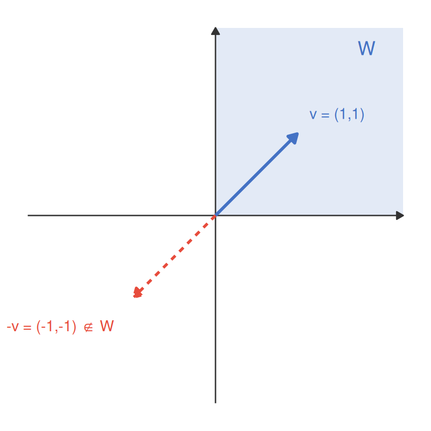
Try it: \(W = \{(x,y)\in\mathbb{R}^2 : x\ge 0,\, y\ge 0\}\)
Take \(v=(1,1)\in W\) and the scalar \(c=-1\). Then
\[c\,v = (-1,-1) \notin W.\]
\(W\) is closed under addition (add two non-negative vectors, you stay non-negative), but it fails closure under scalar multiplication: one axiom is enough to sink the whole structure.
An economic reading
\(W\) is exactly a consumption set \(\{x\ge 0\}\). It’s a cone, not a vector space (one more reason “linear” is doing real work): budget constraints are linear (affine), but the set of feasible bundles generally isn’t closed under scalar multiplication at all.
Span, linear independence, and basis
Span
\[\operatorname{span}(v_1,\ldots,v_k) = \left\{\,\sum_{j=1}^k a_j\,v_j \;\Big|\; a_j\in\mathbb{R}\,\right\}.\]
The span is simply the set of all vectors you can reach using linear combinations of the \(v_j\).
Linear independence
\(\{v_1,\ldots,v_k\}\) are linearly independent iff
\[\sum_j a_j v_j = 0 \implies a_j = 0\;\forall j.\]
In practice: no vector in the family can be expressed as a linear combination of the others.
Basis and dimension
A basis of \(V\) is a linearly independent spanning set: \((v_1,\ldots,v_k)\) are linearly independent and \(\operatorname{span}(v_1,\ldots,v_k) = V\).
\(\dim V\) = number of vectors in any basis of \(V\).
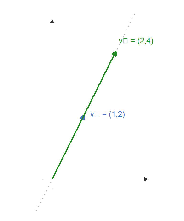
Example: linear dependence in \(\mathbb{R}^2\)
Let \(v_1 = (1,2),\quad v_2 = (2,4)\). We ask: does there exist \(c_1, c_2 \neq (0,0)\) such that \(c_1 v_1 + c_2 v_2 = (0,0)\)?
\[\begin{aligned} c_1 + 2c_2 &= 0,\\ 2c_1 + 4c_2 &= 0. \end{aligned}\]
The first equation gives \(c_1 = -2c_2\). Substituting into the second: \[2(-2c_2) + 4c_2 = -4c_2 + 4c_2 = 0,\] which holds for any \(c_2\). Taking \(c_2 = 1\), we get \(c_1 = -2\), so \[-2\,v_1 + 1\,v_2 = (0,0).\] Therefore \(\{v_1, v_2\}\) is linearly dependent: geometrically, both vectors point along the same line!
Example: linear independence in \(\mathbb{R}^3\)
\(\mathbb{R}^3\): Standard Basis
Take
\[v_1=(1,0,0),\;v_2=(0,1,0),\;v_3=(0,0,1),\quad A=I_3.\]
Then
\[c_1\,v_1 + c_2\,v_2 + c_3\,v_3 = 0 \;\Longleftrightarrow\; \begin{pmatrix}c_1\\c_2\\c_3\end{pmatrix} = 0 \;\Longleftrightarrow\; c_1=c_2=c_3=0,\]
so \(\{v_1,v_2,v_3\}\) is linearly independent. These three vectors form a basis for \(\mathbb{R}^3\), and \(\dim\mathbb{R}^3 = 3\).
Three mutually perpendicular directions, none reachable from the other two (the most standard basis there is).
Dot product and orthogonality
The dot product of two vectors \(\mathbf{u}\) and \(\mathbf{v}\) of size \(n\) is a scalar:
\[\mathbf{u} \cdot \mathbf{v} = \sum_{i=1}^{n} u_i\,v_i = \mathbf{u}^T\mathbf{v} = \mathbf{v}^T\mathbf{u}.\]
Two vectors are orthogonal if and only if \(\mathbf{u} \cdot \mathbf{v} = 0\).
Why do you think we say these vectors are orthogonal?
Geometric interpretation:
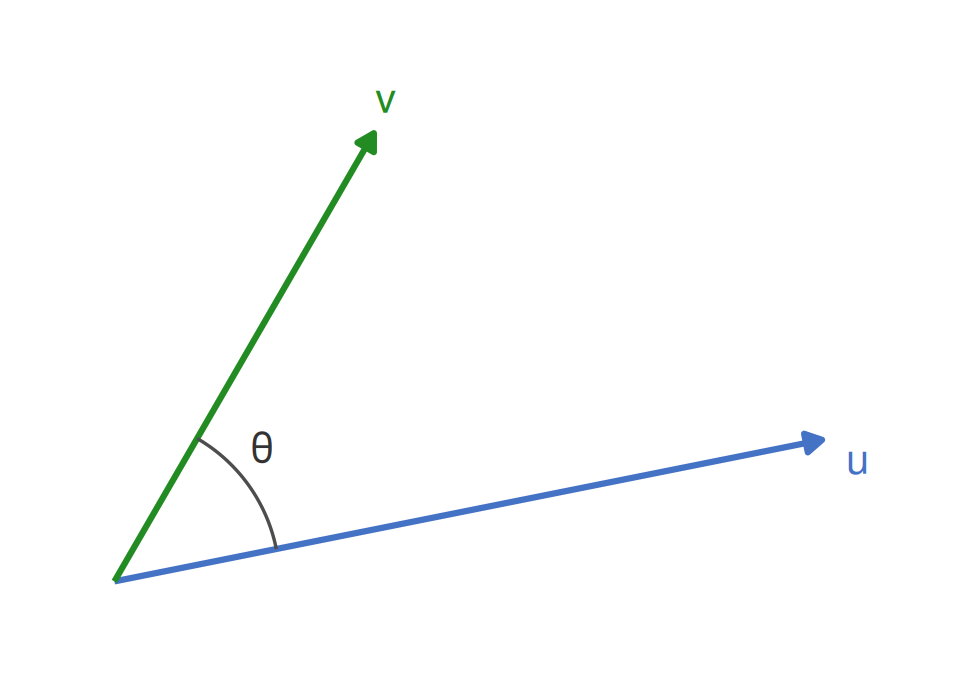
\[\mathbf{u} \cdot \mathbf{v} = \|\mathbf{u}\|\;\|\mathbf{v}\|\;\cos\theta,\]
where \(\theta\) is the angle between them (the law of cosines). Hence
\[\mathbf{u} \cdot \mathbf{v} = 0 \;\Longrightarrow\; \cos\theta = 0 \;\Longrightarrow\; \theta = 90^\circ.\]
An economic implication
When we try to predict test scores with student characteristics, the prediction error \(\hat{\varepsilon}\) we make are orthogonal (unrelated) by construction with student characteristics \(X\): \(X^\top \hat{\varepsilon} = 0\). This geometric fact is the heart of the OLS normal equations.
Orthogonal projection onto a line
Given two vectors that are not orthogonal, how much of one actually points in the direction of the other? In other words, how can we approximate one vector with one other? We start with the simplest version: approximating with a single direction.
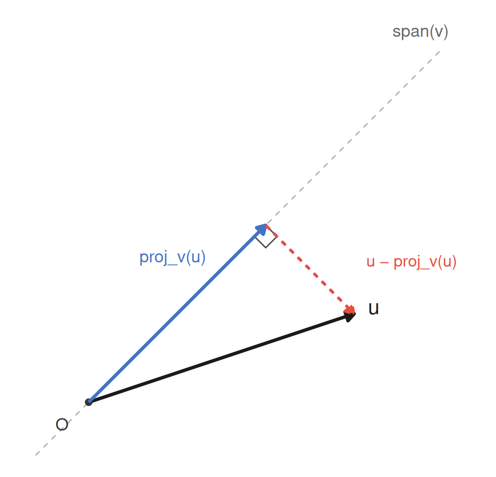
Imagine we have vectors \(u,v \in \mathbb{R}^n\), and we want to find the projection of \(u\) onto \(v\). In practice, this means we want to split \(u\) in 2 parts: a part living in the \(\text{span}(v)\) and one orthogonal to \(v\). Mathematically, how to find it?
Formula for the orthogonal projection
Definition
The orthogonal projection of \(u\) onto the line spanned by \(v \ne 0\) is
\[\operatorname{proj}_v(u) = \frac{u \cdot v}{v \cdot v}\,v.\]
Where does this formula actually come from?
Solve for it directly. \(\operatorname{proj}_v(u)\) has to sit somewhere on the line spanned by \(v\), so it’s some multiple of \(v\) (call it \(cv\)). The one property that pins down \(c\) is that the leftover piece must be perpendicular to \(v\):
\[(u-cv)\cdot v = 0 \;\;\Longrightarrow\;\; u\cdot v = c\,(v\cdot v) \;\;\Longrightarrow\;\; c = \frac{u\cdot v}{v\cdot v}.\]
Would this still work if we wanted to project onto a plane instead of a line?
Orthogonal projection onto a line: example
Worked example
Let \(u=(3,1)\) and \(v=(1,1)\). Then
\[\operatorname{proj}_v(u) = \frac{u\cdot v}{v\cdot v}\,v = \frac{3+1}{1+1}(1,1) = 2(1,1) = (2,2).\]
Residual: \(u - \operatorname{proj}_v(u) = (1,-1)\), and indeed \((1,-1)\cdot(1,1) = 1-1 = 0\). ✓
This is exactly the picture two slides back (same \(u\), same \(v\)), now with the algebra behind it.
Orthogonal projection onto a subspace
A line only lets you move in one direction. The plane \(S\) has two independent directions in it, you can’t eyeball the closest point anymore: you need algebra.
Running example
\[S = \operatorname{span}\{a_1,a_2\} \subset \mathbb{R}^3, \qquad a_1=(1,1,0),\;\; a_2=(0,1,1), \qquad u = (3,2,2).\]
\(u\notin S\): no combination \(c_1a_1+c_2a_2\) can reproduce all three coordinates of \(u\) at once (try it). So: what point in \(S\) is reachable, and closest to \(u\)?
The projection theorem
The projection theorem
For any subspace \(S\subseteq\mathbb{R}^n\) and any \(u\in\mathbb{R}^n\), there is a unique closest point \(\hat u\in S\):
\[\hat u = \operatorname{proj}_S(u) = \operatorname*{arg\,min}_{s\in S}\|u-s\|,\]
and it is completely pinned down by one property (the leftover piece is orthogonal to every vector in \(S\), not just to \(u\)):
\[u-\hat u \;\perp\; S \quad\Longleftrightarrow\quad (u-\hat u)^\top s = 0 \;\;\forall s\in S.\]
A simple demonstration about the “closest point” argument
For any other \(s\in S\): \(\;\|u-s\|^2 = \|u-\hat u\|^2 + \|\hat u - s\|^2 \ge \|u-\hat u\|^2\), because the two pieces are orthogonal. Moving away from \(\hat u\) inside \(S\) can only add distance, never remove it \(\rightarrow\) “closest” and “orthogonal residual” turn out to be the same condition in disguise.
Finding the projection by hand
Write the target as \(\hat u = c_1a_1+c_2a_2\) for unknown weights, stack the spanning vectors into \(A=[a_1\;\;a_2]\), and demand that the residual be orthogonal to both columns of \(A\) at once. (Note that if you are orthogonal to the basis \((a_1,a_2)\) of \(S\), you will be orthogonal to all vectors by construction)
\[A^\top(u-Ac)=0 \quad\Longleftrightarrow\quad \underbrace{A^\top A}_{\text{now a genuine }2\times2}\,c = A^\top u.\]
Plug in the numbers.
\[A = \begin{pmatrix}1&0\\1&1\\0&1\end{pmatrix}, \qquad A^\top A = \begin{pmatrix}2&1\\1&2\end{pmatrix}, \qquad A^\top u = \begin{pmatrix}5\\4\end{pmatrix}.\]
Unlike the line, \(A^\top A\) is not diagonal here: there’s a genuine \(2\times2\) matrix to invert (will study matrix inversion in a few slides but the idea is the same as with numbers, a matrix \(M^{-1}\) is the inverse of \(M\) if \(M^{-1}M = I\)):
\[c = (A^\top A)^{-1}A^\top u = \frac{1}{3}\begin{pmatrix}2&-1\\-1&2\end{pmatrix}\begin{pmatrix}5\\4\end{pmatrix} = \begin{pmatrix}2\\1\end{pmatrix} \;\;\Longrightarrow\;\; \hat u = 2a_1+1a_2 = (2,3,1), \quad u-\hat u = (1,-1,1).\]
The projection matrix p
The steps we just ran (solve \(A^\top A\,c=A^\top u\), then form \(Ac\)) never actually depended on which \(u\) we started with. Bundle them into a single matrix and they work for any \(u\) at once:
\[\hat u = A(A^\top A)^{-1}A^\top u = P_S u, \qquad P_S := A(A^\top A)^{-1}A^\top.\]
For our running example
\[P_S = \frac{1}{3}\begin{pmatrix}2&1&-1\\1&2&1\\-1&1&2\end{pmatrix}.\]
Symmetric by inspection. And \(\operatorname{tr}(P_S) = \tfrac{2+2+2}{3} = 2\) (exactly \(\dim(S)\). Keep that trace fact in your pocket; it resurfaces almost unchanged when we get to OLS.
\(A\) full column rank \(\Rightarrow\) \(A^\top A\) invertible (we’ll see exactly why once we reach positive definite matrices). Two properties of \(P_S\) hold for any subspace, not just ours:
- Idempotent: \(P_S^2=P_S\) (a point already in \(S\) gets sent to itself, so projecting twice changes nothing.
- Symmetric: \(P_S^\top=P_S\) (inherited directly from \(A^\top A\) being symmetric).
Does \(P_S\) change if you pick a different basis for the same subspace \(S\)?
No (and that’s the whole point)
Any two matrices whose columns span the same \(S\) produce the same \(P_S\). The projection depends only on the subspace, never on how you happened to write it down. Remember this formula: in a few slides, \(A\) becomes \(X\) and \(u\) becomes \(Y\): nothing new, just relabelled.
Part ii: linear maps, matrix notation, and rank–nullity
Linear maps and their matrix representation
Every linear map is a matrix
A map \(T:\mathbb{R}^n\to\mathbb{R}^m\) is linear iff \(T(ax+by)=aT(x)+bT(y)\). Any linear map has a matrix representation \(A\in\mathbb{M}_{m\times n}\): \(T(x)=Ax\).
A map is also sometimes called a function.
For instance, \(f(x,y) = \begin{pmatrix} 2x+y\\ x+2y \end{pmatrix}\) is a linear map represented by:
\[A = \begin{pmatrix} 2 & 1 \\ 1 & 2 \end{pmatrix}, \qquad A\begin{pmatrix}x\\y\end{pmatrix} = \begin{pmatrix}2x+y\\x+2y\end{pmatrix}.\]
Why this notation?
- Generalises scalar multiplication: in \(\mathbb{R}^n\to\mathbb{R}^m\), the generalisation is multiplication by a matrix.
- Keeps notation concise. Imagine having to write 68 linear equations with 60 variables…
Matrix notation: two ways to slice the same object
A matrix is just numbers in a grid. What changes everything is how you cut it up (and both cuts show up constantly for the rest of the course.
Reading by columns
\[A = \big[\,c_1(A)\;\; c_2(A)\;\; \cdots \;\; c_n(A)\,\big], \qquad c_j(A) \in \mathbb{R}^m.\]
Reading by rows
\[A = \begin{pmatrix} r_1(A)^\top \\ \vdots \\ r_m(A)^\top \end{pmatrix}, \qquad r_i(A) \in \mathbb{R}^n.\]
Matrix–vector multiplication has two equivalent readings:
\[Ax = \sum_{j=1}^n x_j\, c_j(A) \quad\text{(a weighted sum of columns)}, \qquad (Ax)_i = r_i(A)^\top x \quad\text{(row $i$ dotted with $x$)}.\]
This can be important: some professors like to fill matrices with row vectors, other with column vectors…
If \(X\) is \(N\times K\), what are the sizes of \(c_k(X)\) and \(r_i(X)\)?
Matrix notations
Some researchers (especially in econometrics) also denote matrices as a collection of rows or columns.
For instance, imagine you observe \(K\) characteristics of \(N\) individuals denoted by vectors \(X_1, \ldots, X_N\). You may denote the matrix with all observations as:
\[X = \begin{pmatrix} X_1^\top \\ \vdots \\ \vdots \\ X_N^\top \end{pmatrix} = \begin{pmatrix} X_{11} & X_{12} & \cdots & X_{1K} \\ \vdots & \ddots & &\vdots \\ \vdots & & \ddots & \vdots \\ X_{N1} & X_{N2} & \cdots & X_{NK} \end{pmatrix}\]
The habit that saves you on problem sets
In econometrics, the design matrix \(X\) is \(N\times K\): rows are observations, columns are variables. So \(c_k(X) \in \mathbb{R}^N\) (variable \(k\) across the whole sample) and \(r_i(X) \in \mathbb{R}^K\) (individual \(i\)’s full characteristic vector). Mix the two up (write a row where you meant a column) and every dimension in your derivation silently breaks.
(Have this in mind during spring semester)
Matrix notation: a worked example
\[A = \begin{pmatrix} 1 & 4 \\ 2 & 5 \\ 3 & 6 \end{pmatrix} \qquad (3\times 2).\]
By columns: \(c_1(A) = (1,2,3)\), \(c_2(A) = (4,5,6)\) (each a vector in \(\mathbb{R}^3\)).
By rows: \(r_1(A) = (1,4)\), \(r_2(A) = (2,5)\), \(r_3(A) = (3,6)\) (each a vector in \(\mathbb{R}^2\)).
The two routes agree
For \(x = (1,1)\):
\[Ax = 1\cdot c_1(A) + 1\cdot c_2(A) = (5,7,9)\]
\[Ax = \bigl(r_1(A)^\top x,\; r_2(A)^\top x,\; r_3(A)^\top x\bigr) = (1{+}4,\,2{+}5,\,3{+}6) = (5,7,9).\]
Same matrix, same vector, same answer: two different ways of bookkeeping the exact same computation.
Multiplying two matrices
Definition
If \(A \in \mathbb{M}_{m\times n}\) and \(B \in \mathbb{M}_{n\times p}\), then \(AB \in \mathbb{M}_{m\times p}\) with
\[(AB)_{ij} = r_i(A)^\top c_j(B) = \sum_{k=1}^{n} a_{ik}\,b_{kj}.\]
Entry \((i,j)\) is row \(i\) of \(A\) dotted with column \(j\) of \(B\): exactly the two ways of slicing a matrix from the previous slide, used at the same time. The inner dimensions must match (\(n = n\)); the outer dimensions survive.
What multiplication actually means
\(AB\) is the matrix of the composed map: apply \(B\) first, then \(A\).
\[(AB)x = A(Bx).\]
Everything else follows from this. Associativity \((AB)C = A(BC)\) (composing maps is associative). BUT \(AB \ne BA\) in general. [When is it even defined?{.forestgreen}
Two habits that will save you
- Check dimensions before you compute. \((m\times n)(n\times p) = (m\times p)\). If the inner numbers disagree, the product does not exist: there is no answer to get wrong.
- Order matters, always. \((AB)^\top = B^\top A^\top\), not \(A^\top B^\top\). The reversal is not a typo, and it will come back on the very next slide.
Multiplying two matrices: worked example
\[A = \begin{pmatrix}1&2\\0&1\\3&1\end{pmatrix}\ (3\times 2), \qquad B = \begin{pmatrix}2&0&1\\1&1&0\end{pmatrix}\ (2\times 3) \quad\Longrightarrow\quad AB \text{ is } 3\times 3.\]
\[AB = \begin{pmatrix} 1(2)+2(1) & 1(0)+2(1) & 1(1)+2(0)\\ 0(2)+1(1) & 0(0)+1(1) & 0(1)+1(0)\\ 3(2)+1(1) & 3(0)+1(1) & 3(1)+1(0) \end{pmatrix} = \begin{pmatrix}4&2&1\\1&1&0\\7&1&3\end{pmatrix}.\]
And \(BA\)? Is it even defined? Is it the same size?
\(BA\) is defined, and it is a different object entirely
\(B\) is \(2\times3\) and \(A\) is \(3\times2\), so \(BA\) is \(2\times 2\):
\[BA = \begin{pmatrix}2(1)+0(0)+1(3) & 2(2)+0(1)+1(1)\\ 1(1)+1(0)+0(3) & 1(2)+1(1)+0(1)\end{pmatrix} = \begin{pmatrix}5&5\\1&3\end{pmatrix}.\]
\(AB\) is \(3\times3\), \(BA\) is \(2\times2\): they are not even comparable. Non-commutativity is not an edge case, it is the normal situation.
Block (partitioned) matrices
Sometimes it’s cleaner to chop a matrix into sub-blocks and manipulate the blocks as if they were single numbers.
Partitioning by columns
\[X = \big[\,X_1 \;\; X_2\,\big], \qquad X_1 \in \mathbb{M}_{N\times K_1},\;\; X_2 \in \mathbb{M}_{N\times K_2}.\]
\[X\beta = \big[X_1 \;\; X_2\big]\begin{pmatrix}\beta_1\\ \beta_2\end{pmatrix} = X_1\beta_1 + X_2\beta_2.\]
General \(2\times 2\) block multiplication
\[\begin{pmatrix}A & B \\ C & D\end{pmatrix}\begin{pmatrix}x\\y\end{pmatrix} = \begin{pmatrix}Ax + By \\ Cx + Dy\end{pmatrix},\]
as long as the blocks conform: treat each block exactly like a scalar entry.
Where this comes back today
Split your regressors into a control block \(X_1\) and a variable-of-interest block \(X_2\), and this is exactly the bookkeeping behind the Frisch–Waugh–Lovell theorem you will study in spring semester.
Example: block multiplication by hand
\[X_1 = \begin{pmatrix}1\\1\\1\end{pmatrix}, \qquad X_2 = \begin{pmatrix}1&0\\0&1\\1&1\end{pmatrix}, \qquad \beta_1 = 2,\qquad \beta_2 = \begin{pmatrix}3\\-1\end{pmatrix}.\]
\[X\beta = \big[X_1 \;\; X_2\big]\begin{pmatrix}\beta_1\\ \beta_2\end{pmatrix} = 2\begin{pmatrix}1\\1\\1\end{pmatrix} + \begin{pmatrix}1&0\\0&1\\1&1\end{pmatrix}\begin{pmatrix}3\\-1\end{pmatrix} = \begin{pmatrix}2\\2\\2\end{pmatrix} + \begin{pmatrix}3\\-1\\2\end{pmatrix} = \begin{pmatrix}5\\1\\4\end{pmatrix}.\]
Sanity check
You could also just build \(X = [X_1\;\;X_2]\) as one \(3\times 3\) matrix and multiply by the stacked \(\beta = (2,3,-1)^\top\) directly (block or no block), the answer is the same \((5,1,4)^\top\). Blocks are bookkeeping, not new mathematics.
Image (column space) and rank
Image and kernel of \(f:\mathbb{R}^n\to\mathbb{R}^m\)
- \(\mathrm{Im}(f) = \{f(x)\mid x\in\mathbb{R}^n\}\) (column space): all possible outputs.
- \(\ker(f) = \{x\in\mathbb{R}^n\mid f(x)=0\}\) (null space): inputs that map to zero.
- \(\mathrm{Rank}(f) = \dim(\mathrm{Im}(f))\) = number of linearly independent columns of \(A\).
Using the column decomposition from two slides ago, \(f(x) = Ax = \sum_{j=1}^n x_j\,c_j(A)\), so the image is exactly the span of the columns:
\[\mathrm{Im}(f) = \operatorname{span}\bigl(\{c_1(A),\ldots,c_n(A)\}\bigr).\]
Rank bounds:
- \(\operatorname{Rank}(A) \le n\) (can’t exceed number of columns).
- \(\operatorname{Rank}(A) \le m\) (each column lives in \(\mathbb{R}^m\)).
- Therefore: \(\operatorname{Rank}(A) \le \min\{m, n\}\).
- \(A\) has full rank iff \(\operatorname{Rank}(A) = \min\{m, n\}\).
Example: image, kernel, and rank of a specific matrix
\[A = \begin{pmatrix}1 & 2 & 3\\2 & 4 & 6\end{pmatrix}: \mathbb{R}^3 \to \mathbb{R}^2.\]
Every column is a multiple of \((1,2)\), so
\[\operatorname{Im}(A) = \operatorname{span}\{(1,2)\} \;\Longrightarrow\; \operatorname{Rank}(A) = 1.\]
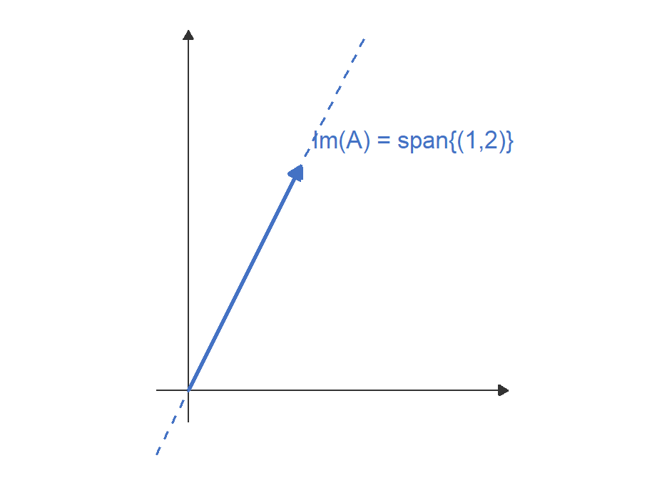
For the kernel, solve \(Ax=0\): since row 2 is just twice row 1, the system reduces to the single equation \(x_1+2x_2+3x_3=0\) (one constraint, three unknowns, so two free parameters):
\[\ker(A) = \operatorname{span}\{(-2,1,0),\,(-3,0,1)\} \;\Longrightarrow\; \dim\ker(A) = 2.\]
Check rank–nullity
\[\operatorname{Rank}(A) + \dim\ker(A) = 1 + 2 = 3 = n. \checkmark\]
Rank–nullity theorem
Theorem (rank–nullity)
For \(f:\mathbb{R}^n\to\mathbb{R}^m\):
\[\underbrace{\operatorname{Rank}(f)}_{\dim(\mathrm{Im}(f))} + \underbrace{\operatorname{Null}(f)}_{\dim(\ker(f))} = \underbrace{n}_{\dim(\operatorname{Domain}(f))}.\]
Intuition (from PlanetMath):
- “Every independent linear constraint takes away one degree of freedom.”
- “\(n\) is the number of unconstrained degrees of freedom.”
- “The nullity is the degrees of freedom remaining in the solution space.”
Degrees of freedom in ols
In OLS with \(N\) observations and \(K\) predictors, residuals \(\hat\varepsilon\) denote the prediction errors you are making. By construction, these errors are orthogonal to \(X\) (an OLS amounts to an orthogonal projection), thus \(\hat\varepsilon\) lies in \(\ker(X^\top)\). By rank–nullity:
\[\mathrm{rank}(X^\top) + \dim(\ker(X^\top)) = N \;\Rightarrow\; \dim(\ker(X^\top)) = N - K.\]
Later, in econometrics, you will see that the variance for the estimation error when you try to predict an outcome \(Y\) with characteristics \(X\) is: \[\hat\sigma^2 = \frac{\hat\varepsilon^\top\hat\varepsilon}{N-K}.\]
The reason why division is by \(N - K\), not \(N\) follows from rank-nullity theorem.
Part iii: solving systems and determinants
Systems of equations as matrices
Consider the system:
\[\begin{cases} a_{11}x_1 + a_{12}x_2 + \cdots + a_{1n}x_n = b_1,\\ \quad\vdots\\ a_{m1}x_1 + a_{m2}x_2 + \cdots + a_{mn}x_n = b_m. \end{cases}\]
Define the coefficient matrix \(A = [a_{ij}]_{m\times n}\), the variable vector \(\mathbf{x} = (x_1,\ldots,x_n)^\top\), and the constant vector \(\mathbf{b} = (b_1,\ldots,b_m)^\top\).
The system compacts to: \[A\mathbf{x} = \mathbf{b}.\]
Rank and solvability
The solution set \(\mathrm{Sol}(b,f) = \{x \mid f(x)=b,\; x \in \mathbb{R}^n\}\)
- is an affine subspace \(x^* + \ker(f)\) of \(\mathbb{R}^n\),
- with dimension equal to the nullity: \(\dim(\mathrm{Sol}(b,f)) = \dim(\ker(f))\).
Rank determines solution structure:
| Condition | Meaning | |
|---|---|---|
| At least one solution for all \(b\) | \(\operatorname{Rank}(f) = m\) | \(f\) is surjective |
| At most one solution for all \(b\) | \(\operatorname{Rank}(f) = n\) | \(f\) is injective |
| Exactly one solution for all \(b\) | \(\operatorname{Rank}(f) = m = n\) | \(f\) is bijective (invertible) |
Invertible function \(\Leftrightarrow\) Invertible associated matrix A \(\Rightarrow\) \(A\) is square (but the converse is false!)
Example: reading the rank table
Three small maps, three outcomes:
\[A_1 = \begin{pmatrix}1&0&0\\0&1&0\end{pmatrix}: \mathbb{R}^3\to\mathbb{R}^2, \qquad A_2 = \begin{pmatrix}1&0\\0&1\\1&1\end{pmatrix}: \mathbb{R}^2\to\mathbb{R}^3, \qquad A_3 = \begin{pmatrix}2&1\\1&2\end{pmatrix}: \mathbb{R}^2\to\mathbb{R}^2.\]
- \(\operatorname{Rank}(A_1) = 2 = m < n\): surjective, not injective (e.g. \((0,0,1) \in \ker(A_1)\)).
- \(\operatorname{Rank}(A_2) = 2 = n < m\): injective, not surjective (its image is only a 2-dimensional plane sitting inside \(\mathbb{R}^3\)).
- \(\operatorname{Rank}(A_3) = 2 = m = n\) (our matrix from before!): bijective (for every \(b\in\mathbb{R}^2\) there is exactly one \(x\) with \(A_3x=b\)).
Rule of thumb
“Wide” matrices (\(n>m\)) can be surjective but never injective: too many inputs collapse onto too few outputs. “Tall” matrices (\(m>n\)) can be injective but never surjective: not enough inputs to reach everywhere. Only square, full-rank matrices can be bijective.
The inverse of a matrix
We want to solve \(A\mathbf{x} = \mathbf{b}\). With ordinary numbers, \(ax = b\) is solved by multiplying both sides by \(1/a\) (and we all know the one case where that fails: \(a=0\)).
What would the matrix version of “\(1/a\)” have to satisfy?
Definition
Let \(A \in \mathbb{M}_{n\times n}\). A matrix \(A^{-1} \in \mathbb{M}_{n\times n}\) is the inverse of \(A\) if
\[A^{-1}A = AA^{-1} = I_n.\]
If such a matrix exists, \(A\) is invertible (or nonsingular), and then
\[A\mathbf{x} = \mathbf{b} \;\;\Longleftrightarrow\;\; \mathbf{x} = A^{-1}\mathbf{b}.\]
The inverse is unique (a one-line proof worth seeing)
Suppose \(B\) and \(C\) both invert \(A\). Then
\[B = B I = B(AC) = (BA)C = I C = C.\]
Nothing but associativity. So “the” inverse is legitimate: there is never more than one.
Only square matrices can have an inverse
\(A^{-1}A\) and \(AA^{-1}\) must both make sense and both equal an identity: this forces \(A\) to be \(n\times n\). This is the algebraic echo of the rank table: only a bijective map can be undone. A \(3\times 2\) matrix maps \(\mathbb{R}^2\) into \(\mathbb{R}^3\) and can never be surjective, so there is nothing to invert.
When does the inverse exist?
Nothing new here: we already have the answer, phrased four different ways. For \(A \in \mathbb{M}_{n\times n}\), the following are equivalent:
The invertibility list
- \(A^{-1}\) exists.
- \(\operatorname{Rank}(A) = n\) (full rank).
- The columns of \(A\) are linearly independent.
- \(\ker(A) = \{0\}\): the only solution of \(Ax = 0\) is \(x = 0\).
- \(A\mathbf{x}=\mathbf{b}\) has exactly one solution for every \(\mathbf{b}\).
- \(\det(A) \ne 0\) (once we reach determinants, two slides from now).
- \(0\) is not an eigenvalue of \(A\) (once we reach Part iv).
Square is necessary, not sufficient
\[A = \begin{pmatrix}1&2\\2&4\end{pmatrix}\]
is perfectly square and has no inverse: its second column is twice the first, so \(\operatorname{Rank}(A)=1<2\) and \((2,-1)^\top \in \ker(A)\). The map squashes the whole plane onto a line, and no matrix can un-squash it: the information is gone.
Properties of the inverse
The rules
For invertible \(A, B \in \mathbb{M}_{n\times n}\) and scalar \(c \ne 0\):
\[(A^{-1})^{-1} = A, \qquad (cA)^{-1} = \tfrac{1}{c}A^{-1}, \qquad (A^\top)^{-1} = (A^{-1})^\top,\]
\[\boxed{(AB)^{-1} = B^{-1}A^{-1}} \qquad \text{(note the reversal!)}\]
Why the order flips: socks and shoes
\(AB\) means “do \(B\), then do \(A\)”. To undo it you must undo the last thing first: take off your shoes, then your socks. Check it algebraically:
\[(AB)(B^{-1}A^{-1}) = A\underbrace{(BB^{-1})}_{I}A^{-1} = AA^{-1} = I. \;\checkmark\]
Try it in the wrong order and the middle does not collapse.
Three things that are false
- \((A+B)^{-1} \ne A^{-1} + B^{-1}\). (Already false for \(1\times1\): \(\tfrac{1}{2+3}\ne\tfrac12+\tfrac13\).)
- \(A^{-1}\) is not “\(A\) with each entry inverted”.
- \(AB = AC\) does not give \(B = C\) unless \(A\) is invertible. There is no cancellation law for singular matrices.
Inverting a \(2\times 2\) matrix
The formula to memorise
\[A = \begin{pmatrix}a&b\\c&d\end{pmatrix} \quad\Longrightarrow\quad A^{-1} = \frac{1}{ad-bc}\begin{pmatrix}d&-b\\-c&a\end{pmatrix}, \qquad \text{provided } ad-bc \ne 0.\]
In words: swap the diagonal entries, flip the sign of the off-diagonal ones, divide by \(ad-bc\). (That quantity \(ad-bc\) is the determinant, which we meet properly in a few slides.)
Worked example: the matrix from Part i
Remember \(A^\top A = \begin{pmatrix}2&1\\1&2\end{pmatrix}\) from the projection example, where we asserted its inverse without justification. Now we can produce it: \(ad-bc = 4-1 = 3\), so
\[\begin{pmatrix}2&1\\1&2\end{pmatrix}^{-1} = \frac{1}{3}\begin{pmatrix}2&-1\\-1&2\end{pmatrix}.\]
Verify: \(\displaystyle \frac13\begin{pmatrix}2&1\\1&2\end{pmatrix}\begin{pmatrix}2&-1\\-1&2\end{pmatrix} = \frac13\begin{pmatrix}3&0\\0&3\end{pmatrix} = I_2.\;\checkmark\)
Always verify. It costs one multiplication and catches every sign error.
The formula does not generalise
There is no comparably short recipe for \(3\times3\) and beyond. For those we need an algorithm: next slide.
The general method: Gauss–Jordan elimination
The recipe
Write \(A\) and \(I\) side by side as one augmented \(n \times 2n\) array, then run row operations (swap rows, scale a row, add a multiple of one row to another) until the left half becomes \(I\):
\[\big[\,A \;\big|\; I\,\big] \;\xrightarrow{\ \text{row operations}\ }\; \big[\,I \;\big|\; A^{-1}\,\big].\]
Whatever the left half becomes, apply the same operations to the right half. If the left half cannot be reduced to \(I\) (a row of zeros appears), then \(A\) is not invertible.
Why on earth does this work?
Each row operation is itself a matrix multiplication on the left by an elementary matrix \(E\). Reducing \(A\) to \(I\) means finding \(E_k \cdots E_2 E_1\) with
\[\underbrace{E_k\cdots E_1}_{=: M} A = I \;\;\Longrightarrow\;\; M = A^{-1}.\]
And what does that same sequence do to the \(I\) sitting in the right half? It produces \(E_k \cdots E_1 I = M = A^{-1}\). The right half is recording the product for you while the left half does the work. Nothing magical: you are building \(A^{-1}\) one row operation at a time.
Worked example (the Sylvester matrix, again)
\[A = \begin{pmatrix}2&1&0\\1&2&1\\0&1&2\end{pmatrix}.\]
\[\left[\begin{array}{ccc|ccc} 2&1&0&1&0&0\\ 1&2&1&0&1&0\\ 0&1&2&0&0&1 \end{array}\right] \xrightarrow[\;R_2 \leftarrow R_2 - R_1\;]{\;R_1 \leftarrow \frac12 R_1\;} \left[\begin{array}{ccc|ccc} 1&\frac12&0&\frac12&0&0\\ 0&\frac32&1&-\frac12&1&0\\ 0&1&2&0&0&1 \end{array}\right]\]
\[\xrightarrow[\;R_1 \leftarrow R_1 - \frac12 R_2,\;\; R_3 \leftarrow R_3 - R_2\;]{\;R_2 \leftarrow \frac23 R_2\;} \left[\begin{array}{ccc|ccc} 1&0&-\frac13&\frac23&-\frac13&0\\ 0&1&\frac23&-\frac13&\frac23&0\\ 0&0&\frac43&\frac13&-\frac23&1 \end{array}\right]\]
\[\xrightarrow[\;R_1 \leftarrow R_1 + \frac13 R_3,\;\; R_2 \leftarrow R_2 - \frac23 R_3\;]{\;R_3 \leftarrow \frac34 R_3\;} \left[\begin{array}{ccc|ccc} 1&0&0&\frac34&-\frac12&\frac14\\ 0&1&0&-\frac12&1&-\frac12\\ 0&0&1&\frac14&-\frac12&\frac34 \end{array}\right]\]
\[\Longrightarrow\quad A^{-1} = \frac14\begin{pmatrix}3&-2&1\\-2&4&-2\\1&-2&3\end{pmatrix}.\]
Sanity check on row 1 of \(A\) against column 1 of \(A^{-1}\): \(\tfrac14\bigl(2(3) + 1(-2) + 0(1)\bigr) = \tfrac44 = 1\). ✓ And note \(A^{-1}\) came out symmetric, as it must: \((A^\top)^{-1}=(A^{-1})^\top\), and \(A=A^\top\) here.
What inversion does geometrically
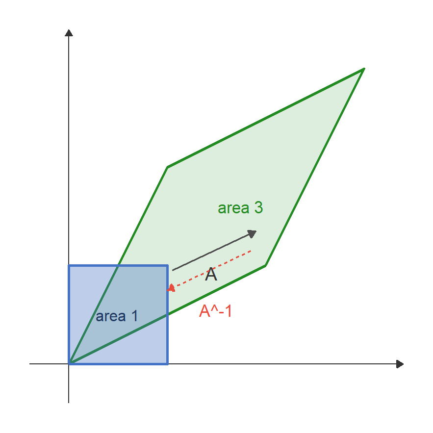
With \(A=\begin{pmatrix}2&1\\1&2\end{pmatrix}\), the unit square (blue) is stretched into the green parallelogram: area \(1 \to 3\).
\(A^{-1}\) is the map that puts it back, so it must shrink area by exactly \(1/3\):
\[\det(A^{-1}) = \frac{1}{\det(A)}.\]
This is why \(\det A = 0\) kills invertibility. If a map flattens area to zero, no map can restore it: you would need to divide by zero.
Application: the leontief input–output model
Motivation: modern economies aren’t a simple chain from raw materials to consumers: industries also sell to each other. Steel producers need electricity to run their furnaces; electricity producers need steel for turbines and pylons. So: how much should each sector produce in total, if we want to satisfy a given level of final consumer demand once every sector’s own input needs are accounted for?
Wassily Leontief won a Nobel Prize for turning exactly this question into a linear algebra problem!
Setting up the model
For each sector \(i\), let:
- \(x_i\) = total output of sector \(i\) (everything it produces, in some common unit),
- \(d_i\) = final demand for sector \(i\)’s output (what households, government, or exporters actually consume: not what other industries buy as inputs),
- \(a_{ij}\) = technical coefficient: units of good \(i\) needed as an input to produce one unit of good \(j\)’s output.
Total output must cover both final demand and everything other sectors need from it as an input:
\[x_i = \underbrace{\sum_j a_{ij}\,x_j}_{\text{used up as input by all sectors}} \;+\; \underbrace{d_i}_{\text{final demand}} \qquad\Longleftrightarrow\qquad x = Ax + d.\]
Why this is not trivial
\(x\) appears on both sides of the equation. Sector 1’s required output depends on sector 2’s output (sector 2 needs steel), and sector 2’s required output depends on sector 1’s (sector 1 needs electricity): which depends on sector 2’s again, and so on. There is no sector you can solve first, and you cannot just “plug in and compute”: it’s a fixed point, not a formula. Exactly the kind of problem linear algebra is built to cut through.
Solving it
Move \(x\) to one side and factor:
\[x - Ax = d \;\;\Longleftrightarrow\;\; (I-A)x = d \;\;\Longleftrightarrow\;\; x = (I-A)^{-1}d,\]
provided \((I-A)\) is invertible. (For a “productive” economy: one that can generate positive final output at all, this holds automatically; you’ll be able to check it yourself once we cover determinants in a few slides.) The matrix \((I-A)^{-1}\) is called the Leontief inverse: it translates a vector of final-demand shocks directly into the total-output response, \(\Delta x = (I-A)^{-1}\Delta d\).
Leontief model: a numeric example
Two sectors: Steel (1) and Electricity (2). Producing one unit of steel requires \(0.2\) units of steel (machinery, inputs) and \(0.4\) units of electricity (to run the furnaces). Producing one unit of electricity requires \(0.3\) units of steel (turbines, pylons) and \(0.1\) units of electricity. Households want \(100\) units of steel and \(50\) units of electricity as final goods:
\[A = \begin{pmatrix}0.2 & 0.3\\0.4 & 0.1\end{pmatrix}, \qquad d = \begin{pmatrix}100\\50\end{pmatrix}.\]
Solve step by step
\[I - A = \begin{pmatrix}0.8 & -0.3\\-0.4 & 0.9\end{pmatrix}.\]
Using the same \(2\times2\) shortcut previewed in Part I (swap the diagonal, flip the off-diagonal signs, divide by \(ad-bc\)):
\[ad-bc = (0.8)(0.9) - (-0.3)(-0.4) = 0.72-0.12 = 0.6, \qquad (I-A)^{-1} = \frac{1}{0.6}\begin{pmatrix}0.9 & 0.3\\0.4 & 0.8\end{pmatrix}.\]
\[x = (I-A)^{-1}d = \frac{1}{0.6}\begin{pmatrix}0.9 & 0.3\\0.4 & 0.8\end{pmatrix}\begin{pmatrix}100\\50\end{pmatrix} = \frac{1}{0.6}\begin{pmatrix}105\\80\end{pmatrix} \approx \begin{pmatrix}175.0\\133.3\end{pmatrix}.\]
Sanity check: does this actually satisfy \(x = Ax+d\)?
\[(Ax)_1 = 0.2(175.0)+0.3(133.3) = 35.0+40.0=75.0, \qquad x_1-(Ax)_1 = 175.0-75.0=100=d_1. \;\checkmark\]
\[(Ax)_2 = 0.4(175.0)+0.1(133.3) = 70.0+13.3=83.3, \qquad x_2-(Ax)_2 = 133.3-83.3=50=d_2. \;\checkmark\]
Exactly \(100\) units of steel and \(50\) of electricity make it to final consumers: the rest was absorbed internally, as inputs to the two sectors themselves.
Reading the multiplier
Steel’s total output (\(175\)) is 75% larger than the final demand it faces (\(100\)), purely because of feedback: producing steel takes electricity, producing that electricity takes steel, and so on. The \((1,1)\) entry of \((I-A)^{-1}\), namely \(0.9/0.6=1.5\), tells you precisely this: one extra dollar of final demand for steel raises total steel output by $1.50. Input–output multipliers like this are exactly how statistical agencies estimate the economy-wide impact of a demand shock hitting a single industry.
Determinant: definition and properties
Definition (informal and hard)
The determinant is the unique map \(\det:\mathbb{M}_{n\times n}\to\mathbb{R}\) that is multilinear in rows, changes sign under row swaps, and satisfies \(\det I = 1\).
Key properties
- \(\det(AB) = \det A \cdot \det B\).
- \(\det(A^\top) = \det A\).
- For triangular matrices: \(\det A = \prod_{i=1}^n a_{ii}\).
- \(\det(cA) = c^n \det A\) for an \(n\times n\) matrix.
The central equivalence
\[\det A \ne 0 \;\iff\; \operatorname{Rank}(A) = n \;\iff\; A \text{ is invertible} \;\iff\; Ax = b \text{ has a unique solution for all } b.\]
Geometric definition of the determinant (i)
\(|\det A|\) = volume scaling factor of the linear map \(A\).
\[A = \begin{pmatrix} 1 & 0 \\ 0 & 1 \end{pmatrix}, \qquad \det(A) = 1.\]
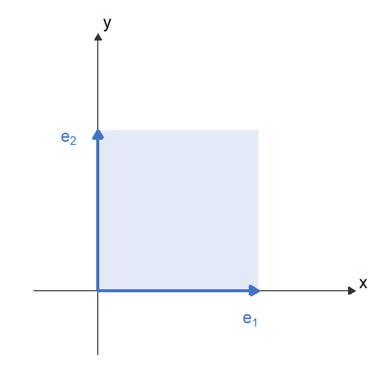
The identity map sends the unit square to itself. The area of a \(1\times 1\) square is \(1 = \det(A)\).
The determinant measures how much the map stretches space.
Geometric interpretation of the determinant (ii)
\[B = \begin{pmatrix} 2 & 0 \\ 0 & 2 \end{pmatrix}, \qquad \det(B) = 4.\]
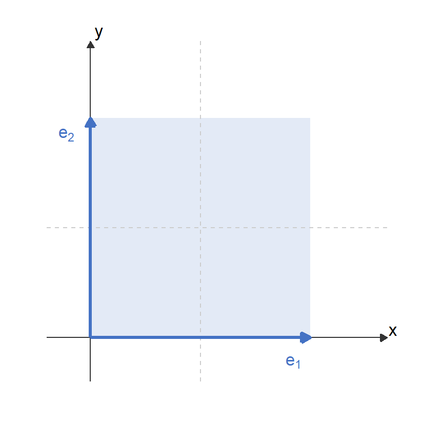
\(B\) doubles every vector: the unit square becomes a \(2\times2\) square.
Area \(= 4 = \det(B)\).
Scaling by \(c\) in each direction multiplies area by \(c^2\) \(\rightarrow\) \(\det(cI_2) = c^2\).
Geometric interpretation of the determinant (iii): orientation
Flipping. \(F = \begin{pmatrix} 0 & 1\\ 1 & 0 \end{pmatrix}\) swaps \(x\) and \(y\).
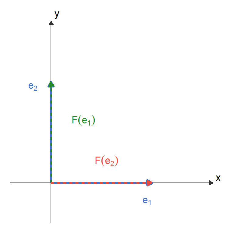
The map preserves area (still a \(1\times1\) square) but reverses orientation (like flipping a transparency sheet).
\[\det(F) = -1.\]
The sign of the determinant encodes orientation, not invertibility. \(F\) is perfectly invertible!
Geometric interpretation of the determinant (iv): squishing
Singular map. \(H = \begin{pmatrix} 0.5 & 0.5\\ -0.5 & -0.5 \end{pmatrix}.\)
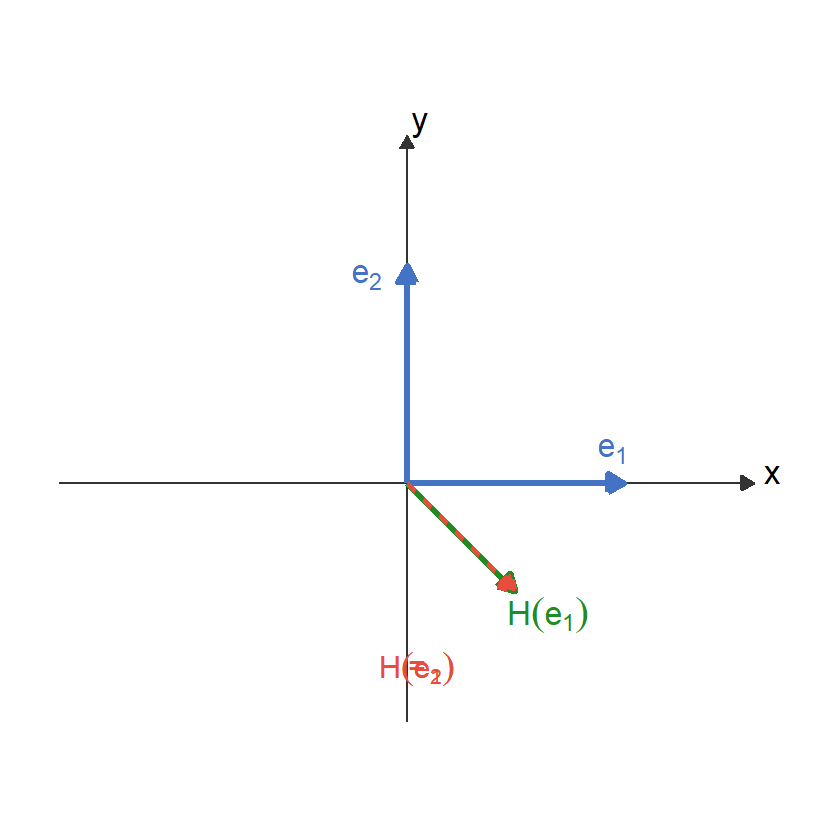
Both basis vectors map to the same point: the whole plane is squashed onto a line.
\[\det(H) = (0.5)(-0.5) - (0.5)(-0.5) = 0.\]
A line has no area: the volume scaling factor is zero.
Not full rank \(\Leftrightarrow\) determinant is zero \(\Leftrightarrow\) not invertible.
Clicker: what does the sign of \(\det A\) tell us?
A \(3\times 3\) matrix \(A\) has \(\det(A) = -8\). Which statement is TRUE?
- A. \(A\) is not invertible because the determinant is negative.
- B. \(A\) is invertible; the map scales volumes by \(8\) and reverses orientation.
- C. \(\det(A^\top) = +8\) (transposing flips the sign).
- D. \(\det(2A) = -16\).
Answer: b
\(\det A \ne 0 \Rightarrow A\) invertible. The sign encodes orientation reversal (a mirror-image effect), not invertibility.
Common mistakes:
- C is wrong: \(\det(A^\top) = \det A = -8\) (transpose preserves determinant).
- D is wrong: \(\det(2A) = 2^3 \det A = 8 \cdot (-8) = -64\).
Invertibility and determinant: full summary
The \(n\times n\) square matrix \(A\) is
invertible (nonsingular) if and only if:
- it has full rank,
- all columns (rows) are linearly independent,
- \(\det(A) \ne 0 \;\Longleftrightarrow\; \operatorname{Rank}(A)=n \;\Longleftrightarrow\; \exists A^{-1}.\)
not invertible (singular) if and only if:
- it is rank-deficient,
- some columns (rows) are linearly dependent,
- \(\det(A) = 0 \;\Longleftrightarrow\; \operatorname{Rank}(A) < n \;\Longleftrightarrow\; \nexists A^{-1}.\)
Bottomline for solving systems
Solving \(A\mathbf{x} = \mathbf{b}\) with a unique solution is equivalent to \(A\) being invertible. When \(A\) is invertible: \(\mathbf{x}^* = A^{-1}\mathbf{b}\).
The cofactor formula for \(A^{-1}\)
Now that we have determinants, we can write \(A^{-1}\) in closed form (no algorithm, just a formula).
Adjugate formula
With cofactors \(C_{ij} = (-1)^{i+j}M_{ij}\) as defined in the appendix, let \(\operatorname{adj}(A) = C^\top\) (the transpose of the cofactor matrix). Then
\[A^{-1} = \frac{1}{\det A}\,\operatorname{adj}(A).\]
For \(n=2\) this collapses to exactly the swap-and-flip rule you already know.
Same matrix, third method
\(A = \begin{pmatrix}2&1&0\\1&2&1\\0&1&2\end{pmatrix}\), with \(\det A = 4\) (computed on the Sylvester slide). The cofactors are
\[C = \begin{pmatrix}3&-2&1\\-2&4&-2\\1&-2&3\end{pmatrix} \;\Longrightarrow\; A^{-1} = \frac14\begin{pmatrix}3&-2&1\\-2&4&-2\\1&-2&3\end{pmatrix},\]
matching Gauss–Jordan exactly.
Never use this to actually compute
The adjugate needs \(n^2\) determinants of size \((n-1)\): catastrophically slow beyond \(3\times3\). Its value is theoretical: it shows that each entry of \(A^{-1}\) is a ratio of polynomials in the entries of \(A\). So \(A \mapsto A^{-1}\) is a smooth function wherever \(\det A \ne 0\) — which is precisely what the implicit function theorem will need when you do comparative statics.
Cramer’s rule
Statement
If \(\det A \ne 0\), the unique solution of \(A\mathbf{x}=\mathbf{b}\) has components
\[x_i = \frac{\det(A_i)}{\det(A)},\]
where \(A_i\) is \(A\) with its \(i\)-th column replaced by \(\mathbf{b}\).
Why economists still teach it
It gives you one unknown without solving for the others, as an explicit ratio of determinants. That is exactly the shape of a comparative-statics answer: “how does the equilibrium interest rate move when government spending rises?” is a question about one coordinate of \(x\), and Cramer hands you a sign you can read off directly from the determinants, without ever inverting anything.
But not for computation
Cramer needs \(n+1\) determinants. For \(n = 20\) this is hopeless; Gauss–Jordan handles it instantly. Use Cramer to reason, never to compute.
Should you ever compute an inverse?
We have spent four slides learning to invert matrices. The truth is: in practice you should almost never do it yourself.
Solving beats inverting
To get \(\mathbf{x}\) from \(A\mathbf{x}=\mathbf{b}\), do not form \(A^{-1}\) and multiply. Solve the system directly (Gaussian elimination / LU / QR under the hood). It is faster and numerically far more stable: forming \(A^{-1}\) does strictly more work than solving, and every extra operation is a chance to accumulate rounding error.
What this means for your econometrics code
\(\hat\beta = (X^\top X)^{-1}X^\top Y\) is how we write OLS, and it is the right way to think about it: the projection formula from Part i. But lm() in R does not compute \((X^\top X)^{-1}\) at all — it uses a QR decomposition of \(X\). The formula is a statement about geometry; the software is doing something equivalent and better conditioned.
Near-singular is the real enemy
\(\det A = 0\) is a knife edge you will essentially never land on exactly with real data. What actually happens is \(\det A \approx 0\): two regressors are nearly collinear, \(X^\top X\) is technically invertible, and \((X^\top X)^{-1}\) has enormous entries. The inverse exists, the computer returns numbers, and those numbers are close to meaningless — huge standard errors, coefficients that swing wildly when you add one observation.
This is multicollinearity, and you now know exactly what it is geometrically: the columns of \(X\) span a subspace, but only barely.
Checking you are alive
\(A\) and \(B\) are invertible \(n\times n\) matrices. Which statement is TRUE?
- A. \((AB)^{-1} = A^{-1}B^{-1}\).
- B. \((A+B)^{-1} = A^{-1}+B^{-1}\).
- C. \((A^\top)^{-1} = (A^{-1})^\top\).
- D. If \(\det A = -3\), then \(A\) is not invertible.
Answer: C
Transpose and inverse commute: take the transpose of \(A^{-1}A = I\) to get \(A^\top (A^{-1})^\top = I\), which says \((A^{-1})^\top\) inverts \(A^\top\).
Common mistakes:
- A forgets the reversal: \((AB)^{-1} = B^{-1}A^{-1}\) (socks and shoes).
- B is false even for \(1\times1\) numbers.
- D confuses sign with vanishing: \(\det A = -3 \ne 0\), so \(A\) is invertible — the negative sign just means the map reverses orientation.
Where inverses show up in economics
You have already seen two
- Leontief: \(x = (I-A)^{-1}d\). The inverse is the multiplier: entry \((i,j)\) says how much sector \(i\) must produce per unit of final demand for \(j\).
- OLS: \(\hat\beta = (X^\top X)^{-1}X^\top Y\). Invertibility of \(X^\top X\) is the full-rank condition, i.e. no perfect multicollinearity.
Coming later
- Comparative statics: equilibrium conditions \(F(x,\theta)=0\) give \(\dfrac{\partial x}{\partial \theta} = -\,J_x^{-1}J_\theta\). Nearly every “what happens if” answer in micro and macro is an inverse Jacobian.
- Markov chains / dynamic systems: \((I-\beta P)^{-1}\) for discounted sums.
The unifying idea
An inverse answers “what input produced this output?” Leontief: what production plan produces this consumption? OLS: what coefficients produce this fitted line? Comparative statics: what change in equilibrium produces this response to a shock? The recurring economic question is inverse by nature, which is why this one operation keeps reappearing all year.
Inverting a block matrix
For a partitioned matrix (using the block notation from Part ii), with \(A\) and the Schur complement \(S = D - CA^{-1}B\) both invertible:
\[\begin{pmatrix}A&B\\C&D\end{pmatrix}^{-1} = \begin{pmatrix} A^{-1}+A^{-1}BS^{-1}CA^{-1} & -A^{-1}BS^{-1}\\ -S^{-1}CA^{-1} & S^{-1} \end{pmatrix}.\]
This is Frisch–Waugh–Lovell in disguise
Split regressors as \(X = [X_1\;\;X_2]\). Then
\[X^\top X = \begin{pmatrix}X_1^\top X_1 & X_1^\top X_2\\ X_2^\top X_1 & X_2^\top X_2\end{pmatrix},\]
and the Schur complement of the top-left block is \(X_2^\top X_2 - X_2^\top X_1 (X_1^\top X_1)^{-1}X_1^\top X_2 = X_2^\top M_{X_1} X_2\): the variation in \(X_2\) left over after partialling out \(X_1\). The bottom-right block of the inverse then delivers \(\hat\beta_2\) from residualised data alone. FWL is not a separate theorem so much as one corner of this formula.
Part iv: eigenvalues and diagonalisation
Motivation and applications
Disclaimer
You will not use eigenvalues and eigenvectors heavily in the fall term (only a bit in macro). However, they are essential if you want to understand machine learning or dig into advanced econometrics.
Key use cases in economics:
- Dynamic systems stability (e.g., Solow model, Blanchard–Kahn conditions)
- Principal component analysis (PCA) for dimensionality reduction
- Markov chains and long-run stationary distributions
- Leontief input–output multipliers
Eigenvalues and eigenvectors: definitions
Eigenvector
A nonzero vector \(v\) such that \(Av = \lambda v\) is an eigenvector of \(A\). It is a vector whose direction is unchanged after applying \(A\): only its length (and possibly sign) changes.
Eigenvalue
The scalar \(\lambda\) satisfying \(Av = \lambda v\) is the corresponding eigenvalue.
Key Theorem
The eigenvalues of \(A\) are the roots of the characteristic polynomial:
\[\det(A - \lambda I) = 0.\]
For each eigenvalue \(\lambda\), the eigenvectors are the nonzero solutions to: \[(A - \lambda I)v = 0.\]
Geometric interpretation of eigenvectors
\[A = \begin{pmatrix}2 & 1\\1 & 2\end{pmatrix}: \quad f\bigl([x,y]^\top\bigr) = \begin{pmatrix}2x+y\\x+2y\end{pmatrix}.\]
Eigenvectors satisfy \(f(v) = \lambda v\): direction preserved, only scaled.
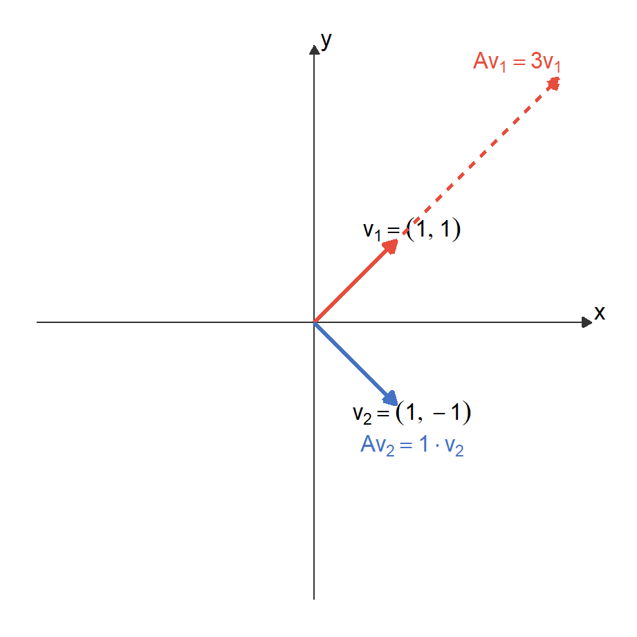
\(v_1\) is scaled by \(3\) (stretched); \(v_2\) is unchanged (\(\lambda_2 = 1\)). Both keep their direction.
Computing eigenvalues and eigenvectors
Step 1: Form \(A - \lambda I\). Step 2: Solve \(\det(A - \lambda I) = 0\). Step 3: Find \(v\) for each \(\lambda\).
Example with \(A = \begin{pmatrix}2 & 1 \\ 1 & 2\end{pmatrix}\):
\[\det(A - \lambda I) = \det\begin{pmatrix}2-\lambda & 1\\1 & 2-\lambda\end{pmatrix} = (2-\lambda)^2 - 1 = \lambda^2 - 4\lambda + 3 = (\lambda-3)(\lambda-1) = 0.\]
Eigenvalues: \(\lambda_1 = 3\), \(\lambda_2 = 1\).
For \(\lambda_1 = 3\): \((A - 3I)v = \begin{pmatrix}-1&1\\1&-1\end{pmatrix}v = 0 \Rightarrow v_1 = (1,1)^\top\).
For \(\lambda_2 = 1\): \((A - I)v = \begin{pmatrix}1&1\\1&1\end{pmatrix}v = 0 \Rightarrow v_2 = (1,-1)^\top\).
Diagonalisation
Definition
\(A\) is diagonalizable if there exists an invertible \(P\) such that: \[P^{-1}AP = D = \operatorname{diag}(\lambda_1,\ldots,\lambda_n).\]
Theorem
\(A\) is diagonalizable iff \(A\) has \(n\) linearly independent eigenvectors. The eigenvectors are the columns of \(P\); eigenvalues are the diagonal entries of \(D\).
Why does this matter?
\[A^k = P\,\operatorname{diag}(\lambda_1^k,\ldots,\lambda_n^k)\,P^{-1}.\]
Computing \(A^{100}\) becomes trivial: just raise each eigenvalue to the 100th power. This is the key to solving dynamic systems: \(x_t = A^t x_0\).
Determinant via eigenvalues
\[\det(A) = \prod_{i=1}^n \lambda_i, \qquad \operatorname{tr}(A) = \sum_{i=1}^n \lambda_i.\]
\(A\) is invertible iff all eigenvalues are nonzero.
Example: diagonalising our running matrix
Recall \(A=\begin{pmatrix}2&1\\1&2\end{pmatrix}\) with \(\lambda_1=3,\,v_1=(1,1)\) and \(\lambda_2=1,\,v_2=(1,-1)\).
\[P = \begin{pmatrix}1&1\\1&-1\end{pmatrix}, \qquad D = \begin{pmatrix}3&0\\0&1\end{pmatrix}, \qquad P^{-1} = \frac{1}{2}\begin{pmatrix}1&1\\1&-1\end{pmatrix}.\]
You can check \(P^{-1}AP=D\) by direct multiplication (a good five-minute hand exercise).
The payoff: compute \(A^2\) two ways.
\[A^2 = \begin{pmatrix}2&1\\1&2\end{pmatrix}^2 = \begin{pmatrix}5&4\\4&5\end{pmatrix} \qquad\text{(direct multiplication)}\]
\[A^2 = PD^2P^{-1} = \frac{1}{2}\begin{pmatrix}1&1\\1&-1\end{pmatrix}\begin{pmatrix}9&0\\0&1\end{pmatrix}\begin{pmatrix}1&1\\1&-1\end{pmatrix} = \begin{pmatrix}5&4\\4&5\end{pmatrix}. \checkmark\]
Same idea, 100 steps later
Both routes take similar effort for \(A^2\). But \(A^{100}\) directly means 99 matrix multiplications; via \(PD^{100}P^{-1}\) it’s three matrix multiplications and raising two numbers to the 100th power.
Part v: positive definite matrices
Positive definite matrices
Definition
A symmetric matrix \(Q \in \mathbb{M}_{n\times n}\) is:
- Positive definite (PD): \(x^\top Qx > 0\) for all \(x \ne 0\).
- Positive semidefinite (PSD): \(x^\top Qx \ge 0\) for all \(x\).
- Negative definite (ND): \(x^\top Qx < 0\) for all \(x \ne 0\).
- Negative semidefinite (NSD): \(x^\top Qx \le 0\) for all \(x\).
\(Q\) is PD iff all eigenvalues are strictly positive. \(Q\) is PSD iff all eigenvalues are non-negative.
\(X^\top X\) is always psd
For any vector \(v\): \(\;v^\top X^\top X v = \|Xv\|^2 \ge 0\).
It is PD (hence invertible) iff \(\ker(X) = \{0\}\), i.e. columns of \(X\) are linearly independent. This is exactly the full rank condition required for OLS to have a unique solution.
Example: testing definiteness by hand
\[Q_1 = \begin{pmatrix}2&0\\0&3\end{pmatrix}, \qquad Q_2 = \begin{pmatrix}1&2\\2&1\end{pmatrix}.\]
For \(Q_1\): \(x^\top Q_1 x = 2x_1^2+3x_2^2 > 0\) for any \(x\ne 0\): clearly positive definite (a diagonal matrix with positive entries is the easy case).
For \(Q_2\), try two test vectors: \(x=(1,0) \Rightarrow x^\top Q_2 x = 1 > 0\), but \(x=(1,-1) \Rightarrow x^\top Q_2 x = -2 < 0\). The sign flips: \(Q_2\) is indefinite.
The problem with testing vectors one at a time
Plugging in vectors can rule a matrix out the moment you find two with opposite signs, but it can never fully confirm PD: there are infinitely many directions to check. We need a finite, mechanical test: Sylvester’s criterion, next.
Sylvester’s criterion
Theorem (sylvester’s criterion)
Let \(Q \in \mathbb{M}_{n\times n}\) be symmetric. Let \(\Delta_k = \det(Q_{1:k,\,1:k})\) be the \(k\)-th leading principal minor.
- \(Q\) positive definite \(\iff\) \(\Delta_k > 0\) for all \(k = 1,\ldots,n\).
- \(Q\) negative definite \(\iff\) \(\operatorname{sign}(\Delta_k) = (-1)^k\) for all \(k\).
Worked example
\[Q = \begin{pmatrix}2&1&0\\1&2&1\\0&1&2\end{pmatrix} \quad\Longrightarrow\quad \Delta_1 = 2,\quad \Delta_2 = \det\begin{pmatrix}2&1\\1&2\end{pmatrix}=3,\quad \Delta_3=\det(Q)=4.\]
All three positive \(\Rightarrow\) \(Q\) is positive definite (no eigenvalues needed, no test vectors, just three small determinants.
Why this matters
Sylvester gives a fast way to check PD/ND for small matrices: compute a few determinants rather than finding all eigenvalues.
You will use this constantly in second-order conditions for constrained optimisation.
Connection to optimisation
At a critical point \(\nabla f(x^*) = 0\): \[f(x^* + \Delta x) - f(x^*) \approx \tfrac{1}{2}(\Delta x)^\top H_f(x^*)\Delta x.\]
- \(H_f(x^*)\) negative definite \(\Rightarrow\) strict local maximum.
- \(H_f(x^*)\) positive definite \(\Rightarrow\) strict local minimum.
- \(H_f(x^*)\) indefinite \(\Rightarrow\) saddle point.
Exercise: negative definiteness
A symmetric \(3\times 3\) matrix \(Q\) has leading principal minors \(\Delta_1 = -2\), \(\Delta_2 = 3\), \(\Delta_3 = -5\). What can you conclude?
- A. \(Q\) is positive definite.
- B. \(Q\) is negative definite.
- C. \(Q\) is indefinite (neither PD nor ND).
- D. \(Q\) is positive semidefinite.
Answer: b (negative definite)
By Sylvester’s criterion: \(Q\) ND \(\iff\) signs alternate as \((-1)^1, (-1)^2, (-1)^3\), i.e. \(-, +, -\).
Here \(\Delta_1 = -2 < 0\), \(\Delta_2 = 3 > 0\), \(\Delta_3 = -5 < 0\). ✓
All eigenvalues of \(Q\) are strictly negative: the quadratic form \(x^\top Qx < 0\) for all \(x \ne 0\).
Part vi: OLS as a projection
OLS as a projection
Imagine you want to decompose a quantity \(Y \in \mathbb{R}^N\) into two parts: one part explained by the matrix
\(X \in \mathbb{M}_{N\times K}\) having full column rank and another part orthogonal to \(X\).
What is the tool we studied that allows to answer this question?
The projection matrix!
Derivation
Since \(X\) has full column rank, \(X^\top X\) is PD (hence invertible) and we can find some vector \(\hat\beta \in \mathbb{R}^K\) \[\hat\beta = (X^\top X)^{-1} X^\top Y.\] such that \(Y = X\beta + \epsilon = \underbrace{X(X^\top X)^{-1} X^\top}_{P_X} Y + \epsilon\)
with \(\epsilon\) being the orthogonal part to \(X\)
Geometric interpretation
\(\hat Y = X\hat\beta = X(X^\top X)^{-1}X^\top Y = P_X Y\) is the orthogonal projection of \(Y\) onto \(\operatorname{col}(X)\).
Residuals \(\hat\varepsilon = (I - P_X)Y\) are perpendicular to all regressors: \(X^\top \hat\varepsilon = 0\).
During your econometrics journey, you will discover conditions under which \(\beta\) gives you the causal effect of \(X\) on \(Y\).
The projection matrix \(P_X\)
Definition and properties
\[P_X = X(X^\top X)^{-1}X^\top, \qquad M_X = I - P_X \quad \text{(annihilator)}.\]
| Property | \(P_X\) | \(M_X\) |
|---|---|---|
| Symmetric | \(P_X^\top = P_X\) | \(M_X^\top = M_X\) |
| Idempotent | \(P_X^2 = P_X\) | \(M_X^2 = M_X\) |
| Rank | \(K\) | \(N-K\) |
| Eigenvalues | \(0\) and \(1\) only | \(0\) and \(1\) only |
Same object, new letters
This is exactly the general projection matrix \(P_S = A(A^\top A)^{-1}A^\top\) from Part I, with \(A = X\) and \(S = \operatorname{col}(X)\). Nothing new to memorise here: just relabelled.
Trace and degrees of freedom
\[\operatorname{tr}(P_X) = K, \qquad \operatorname{tr}(M_X) = N-K.\]
The trace of an idempotent matrix equals its rank. The \(N - K\) comes directly from rank–nullity (connecting back to Part I).
Example: ols by hand with three data points
Let \(X=(1,2,3)^\top\) (a single regressor, no intercept) and \(Y=(2,2,4)^\top\).
\[\hat\beta = \frac{X^\top Y}{X^\top X} = \frac{1\cdot 2+2\cdot 2+3\cdot 4}{1^2+2^2+3^2} = \frac{18}{14} = \frac{9}{7} \approx 1.29.\]
\[\hat Y = X\hat\beta = \Big(\tfrac{9}{7},\tfrac{18}{7},\tfrac{27}{7}\Big), \qquad \hat\varepsilon = Y-\hat Y = \Big(\tfrac{5}{7},-\tfrac{4}{7},\tfrac{1}{7}\Big).\]
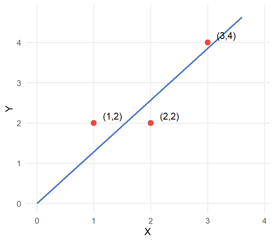
Orthogonality check: \(X^\top\hat\varepsilon = 1\cdot\tfrac{5}{7} + 2\cdot(-\tfrac{4}{7}) + 3\cdot\tfrac{1}{7} = \tfrac{5-8+3}{7} = 0.\) ✓
What \(P_X\) looks like here
\[P_X = X(X^\top X)^{-1}X^\top = \frac{1}{14}\begin{pmatrix}1&2&3\\2&4&6\\3&6&9\end{pmatrix}, \qquad \operatorname{tr}(P_X) = \frac{1+4+9}{14} = 1 = K,\]
exactly \(K=1\) regressor, exactly as the table on the previous slide promised.
Wrap-up
Session 2: key takeaways
Foundations
- Vector spaces: basis, dimension, span are the vocabulary of multivariate statistics.
- Projections: every projection matrix, from a line to \(P_X\), is \(A(A^\top A)^{-1}A^\top\).
- Rank–Nullity: explains degrees of freedom in OLS and the geometry of column spaces.
- Determinants: encode invertibility; \(|\det A|\) measures volume scaling; sign encodes orientation.
Tools
- Eigenvalues: control stability of dynamic systems; spectral criterion for PD matrices.
- PD matrices: \(X^\top X\) PD \(\iff\) unique OLS solution; Hessian PD \(\iff\) strict local minimum.
- OLS = projection: \(\hat\beta\) projects \(Y\) onto \(\operatorname{col}(X)\); residuals are orthogonal to all regressors.
Looking ahead
Session 3 introduces integration and its connection to probability. The OLS geometry you built today will return when we discuss the spectral theorem and constrained optimisation in later sessions.
Resources
General resources
- 3Blue1Brown: Essence of Linear Algebra (YouTube, highly recommended visual introduction)
- Simon & Blume, Chapters 10–17
- Gilbert Strang, Introduction to Linear Algebra (MIT OpenCourseWare, free)
For the tutorial session
Exercises will cover:
- Checking linear independence and finding a basis.
- Computing determinants and verifying invertibility.
- Finding eigenvalues and classifying stability of a 2D system.
- Verifying Sylvester’s criterion on a \(3\times 3\) Hessian.
- Deriving \(\hat\beta\) and verifying \(X^\top\hat\varepsilon = 0\).
- Applying FWL: manually partial out a control and verify coefficient equality.
Appendix
Gaussian elimination
How to reduce \(A\) to row echelon form \(A'\):
For \(i = 1\) to \(n\):
- If \(a_{ii} = 0\):
- If all entries in column \(i\) below \(a_{ii}\) are zero, advance to \(i+1\).
- Otherwise: swap row \(i\) with the first row \(i'\) that has a nonzero \(a_{i'i}\); multiply the new row \(i\) by \(-1\) to preserve the determinant.
- If \(a_{ii} \ne 0\):
- Pivot on all rows \(i' > i\): add \(-\tfrac{a_{i'i}}{a_{ii}}\) times row \(i\) to row \(i'\), making all entries below \(a_{ii}\) equal to zero.
- If \(a_{ii} = 0\):
Row echelon form and solutions
The row echelon form tells us:
- Consistent (at least one solution): rank of augmented matrix \(=\) rank of \(A\).
- Exactly one solution: rank of \(A = n\); every row of \(A'\) has at least one nonzero entry; kernel dimension is zero.
- Infinitely many solutions: rank of \(A < n\); at least one row of \(A'\) is all-zero; kernel dimension \(> 0\).
Recursive computation of the determinant
For each entry \(a_{ij}\) of \(A\), define the minor \(M_{ij} = \det(A^{-(i,j)})\), where \(A^{-(i,j)}\) is \(A\) with row \(i\) and column \(j\) removed.
Define the cofactor \(C_{ij} = (-1)^{i+j} M_{ij}\).
Laplace’s expansion along row \(i\):
\[\det(A) = \sum_{j=1}^n a_{ij}\,C_{ij} = \sum_{j=1}^n a_{ij}\,(-1)^{i+j}\,\det(A^{-(i,j)}).\]
Warning
Laplace’s formula requires \(\sim n!\) operations: impractical for large \(n\). Prefer LU decomposition in practice.
Strang, Gilbert. 2005. “MIT 18.06 Linear Algebra, Spring 2005.” YouTube Playlist. MIT OpenCourseWare. https://www.youtube.com/playlist?list=PLE7DDD91010BC51F8.
Strang, Gilbert. 2023. Introduction to Linear Algebra. 6th ed. Wellesley-Cambridge press.